Overview of the Excel SUMPRODUCT Function
The SUMPRODUCT function is a powerful tool in Excel that allows you to calculate the sum of products of corresponding values from one or more arrays. Here are the key points:
Basic Use:
- To find the sum of products, multiply corresponding numbers in different ranges and add up the results.
- For instance, if you have data like {2, 3, 4} in one list and {5, 10, 20} in another, applying SUMPRODUCT yields 120 (because (2 \times 5 + 3 \times 10 + 4 \times 20 = 120))
Syntax:
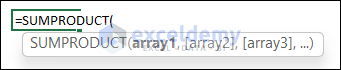
The Syntax of the SUMPRODUCT function is:
=SUMPRODUCT(array1,[array2],[array3],…)
You can provide one or more arrays as arguments.
Argument:
| Argument | Required or Optional | Value |
|---|---|---|
| array 1 | Required | The first array of numbers. |
| [array2] | Optional | The second array of numbers. |
| [array3] | Optional | The third array of numbers. |
Return Value:
It returns the sum of the products of the corresponding values from all the arrays.
Note:
- All arrays must have the same dimensions; otherwise, Excel displays a #VALUE! error.
- If any cell within an array contains non-numeric text, SUMPRODUCT treats it as 0.
- If an array contains Boolean values (TRUE and FALSE), you can convert it to an array of numbers using “–”. For example, –{TRUE, FALSE, TRUE, TRUE, FALSE} becomes {1, 0, 1, 1, 0}.
Dataset Overview
Let’s assume we have a dataset of student records of Saint Xavier’s school containing 3 columns named Student Name, Marks in Physics, and Marks in Chemistry.

We need to find the count or total numbers according to different criteria using the SUMPRODUCT function.
Example 1 – Counting Cells with Specific Criteria
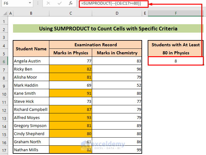
Suppose you want to calculate how many students scored 80 or above in Physics. Follow these steps:
- Click on cell F6.
- Insert the formula:
=SUMPRODUCT(--(C6:C17>=80))Formula Breakdown:
- (C6:C17 >= 80) checks each cell in the range C6:C17. If it’s greater than or equal to 80, it returns TRUE; otherwise, FALSE.
- –(C6:C17 >= 80) converts TRUE/FALSE to 1/0.
- The result is 8, representing the number of students who achieved at least 80 in Physics.
- Press Enter.
Example 2 – Counting Cells with Multiple Criteria (AND Type)
Let’s count the total number of students with at least 80 in both Physics and Chemistry:
- Click on cell F6.
- Insert the formula:
=SUMPRODUCT(--(C6:C17>=80),--(D6:D17>=80))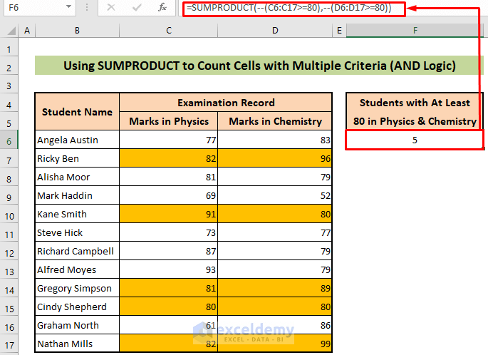
Formula Breakdown:
- –(C6:C17 >= 80) gives an array of 1s and 0s (1 for scores >= 80 in Physics).
- –(D6:D17 >= 80) gives a similar array for Chemistry.
- Multiplying these arrays yields {0, 1, 0, 0, 1, 0, 0, 0, 1, 1, 0, 1}.
- The sum of this array is 5, representing students with at least 80 in both subjects.
Example 3 – Counting Cells with Multiple Criteria (OR Type)
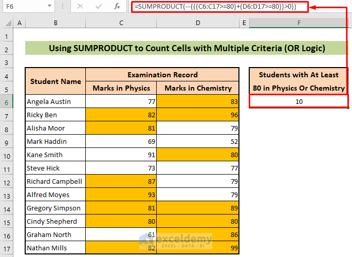
Suppose you want to count the total number of students who scored at least 80 in either Physics or Chemistry (or both). Follow these steps:
- Click on cell F6.
- Insert the formula:
=SUMPRODUCT(--(((C6:C17>=80)+(D6:D17>=80))>0))Formula Breakdown:
- (C6:C17 >= 80) checks each cell in the range C6:C17. If it’s greater than or equal to 80, it returns TRUE; otherwise, FALSE.
- (D6:D17 >= 80) does the same for Chemistry.
- (C6:C17 >= 80) + (D6:D17 >= 80) adds these two Boolean arrays, resulting in an array with values 0, 1, or 2.
- ((C6:C17 >= 80) + (D6:D17 >= 80)) > 0 converts this array to TRUE (when the value is greater than 0) or FALSE (when the value is 0).
- –(((C6:C17 >= 80) + (D6:D17 >= 80)) > 0) converts TRUE/FALSE to 1/0.
- The result is 10, representing the number of students with at least 80 in either subject.
- Press Enter.
Read More: SUMPRODUCT for Counting with Multiple Criteria in Excel
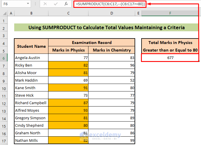
Example 4 – Calculating Total Marks with a Criteria
Suppose you want to calculate the total marks of students in Physics, considering only marks greater than or equal to 80:
- Click on cell F6.
- Insert the formula:
=SUMPRODUCT(C6:C17,--(C6:C17>=80))Formula Breakdown:
- C6:C17 contains the marks in Physics.
- –(C6:C17 >= 80) converts TRUE/FALSE to 1/0.
- The result is 677, which is the total marks of students with scores of at least 80 in Physics.
- Press Enter.
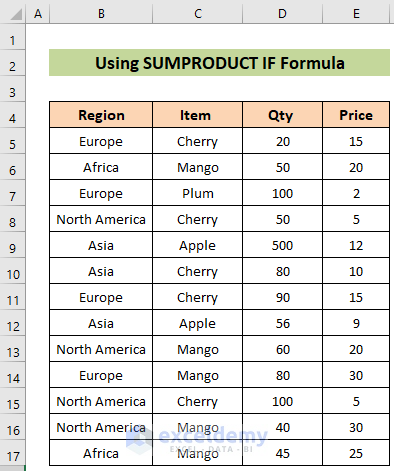
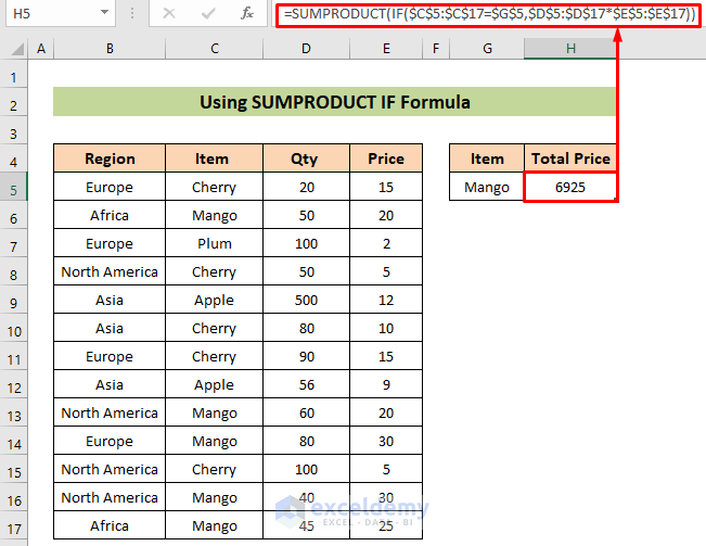
Example 5 – Using SUMPRODUCT-IF for Specific Criteria
Suppose you have sales data with item names, quantities, and unit prices. You want to find the total price of a specific item. Follow these steps:
- Insert the desired item’s name in cell G5.
- Click on cell H5 and insert the formula:
=SUMPRODUCT(IF($C$5:$C$17=$G$5,$D$5:$D$17*$E$5:$E$17))- Explanation:
- IF($C$5:$C$17 = $G$5, $D$5:$D$17 * $E$5:$E$17) multiplies quantity and unit price only for the specified item.
- The result is 6925, representing the total price of the special item.
- Press Enter.
Read More: How to Use SUMPRODUCT with Criteria in Excel
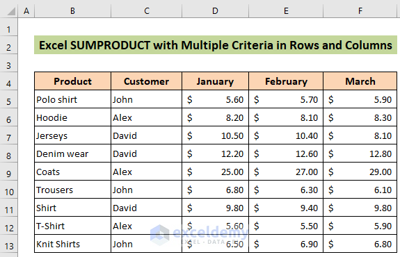
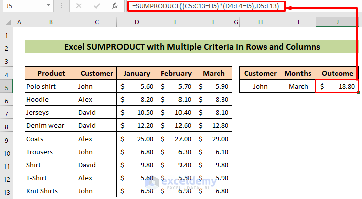
Example 6 – SUMPRODUCT with Multiple Criteria in Rows and Columns
Suppose you have a dataset of products with customer names and prices for January, February, and March. You want to calculate the total sales based on specific criteria. Follow these steps:
- Insert your desired criteria in cells H5 and I5.
- Click on cell J5 and insert the formula:
=SUMPRODUCT((C5:C13=H5)*(D4:F4=I5),D5:F13)- Explanation:
- (C5:C13 = H5) checks if the customer’s name matches the desired criteria.
- (D4:F4 = I5) checks if the month matches the desired criteria.
- (C5:C13 = H5) * (D4:F4 = I5) multiplies these Boolean arrays.
- The result is the total sales based on the specified criteria.
- Press Enter.
Read More: How to use SUMPRODUCT Function with Multiple Columns in Excel
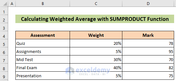
Example 7 – Calculating Weighted Average
Suppose you have a dataset of student grading systems, including the weight of assessments and the marks obtained by each student. You want to calculate the weighted average for an individual. Follow these steps:
- Click on the merged cell E5.
- Insert the formula:
=SUMPRODUCT(C5:C9*D5:D9)/SUM(C5:C9)- Explanation:
- C5:C9 contains the weights of assessments.
- D5:D9 contains the corresponding marks obtained.
- SUMPRODUCT(C5:C9 * D5:D9) calculates the sum of products of weights and marks.
- SUM(C5:C9) gives the total weight.
- The result is a weighted average of 77.9 in cell E5.
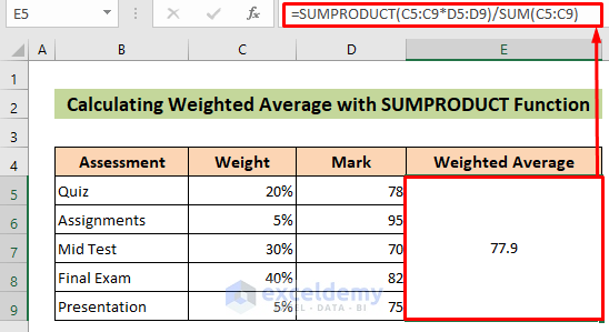
You will get a weighted average of 77.9 in cell E5.
Things to Remember
- Remember that if an argument is of the wrong data type (not an array), Excel displays an #VALUE! error
Download Practice Workbook
You can download the practice workbook from here:
Excel SUMPRODUCT Function: Knowledge Hub
<< Go Back to Excel Functions | Learn Excel
Get FREE Advanced Excel Exercises with Solutions!
