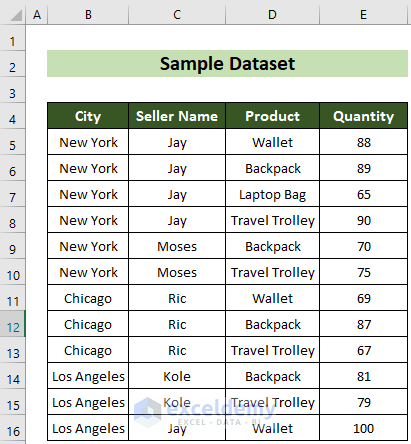
Below is a sales report dataset containing 4 columns: City, Seller Name, Product, and Quantity. We want to sum the quantity of the products according to multiple criteria.
Method 1 – Apply Multiple Criteria with OR Logic Operation Using the SUMPRODUCT Function
1.1. Using the Single SUMPRODUCT Function
Steps:
- Insert your criteria in cells G5 and H5.
- Click on cell I5 and insert the formula below:
=SUMPRODUCT(((B5:B16=G5)+(D5:D16=H5))*E5:E16)- Press Enter.
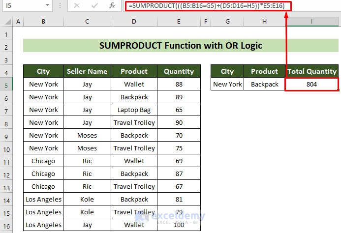
As a result, you will get the total quantity for the products from New York or the product being Backpack.
Read More: How to Use SUMPRODUCT with Criteria in Excel
1.2. Using Multiple SUMPRODUCT Functions
Steps:
- Insert your required criteria in cells G5 and H5.
- Click on cell I5 and insert the formula below:
=SUMPRODUCT((B5:B16=G5)*E5:E16)+SUMPRODUCT((D5:D16=H5)*E5:E16)- Press Enter.
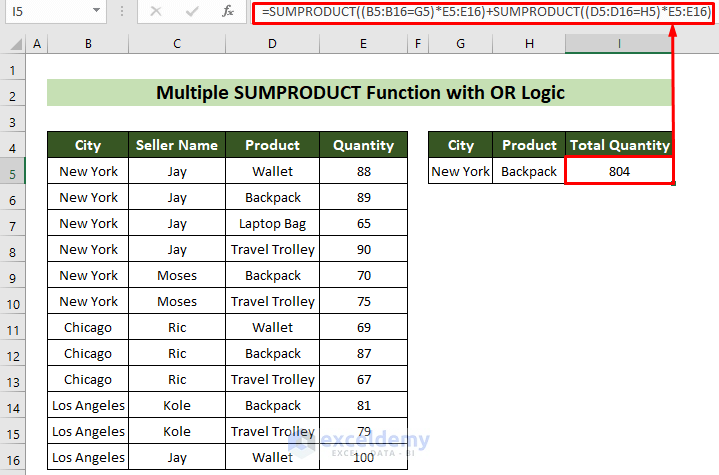
As a result, two SUMPRODUCT functions will work together, and we will get our total quantity for products from New York or the backpack product.
Read More: How to Use SUMPRODUCT Function with Multiple Columns in Excel
Method 2 – Apply Multiple Criteria with AND Logic Operation Using SUMPRODUCT Function
Steps:
- Click on cells G5 and H5 and insert your multiple criteria.
- Click on cell I5.
- Insert the following formula and press the Enter key.
=SUMPRODUCT((B5:B16=G5)*(D5:D16=H5)*E5:E16)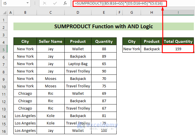
Thus, we will get the desired result for the New York City Backpack’s total quantity.
Note: We can write the formula in another way. That approach is using two unary (-) operators ahead of the array_criteria. So, the formula would be: =SUMPRODUCT((--(B5:B16=G5))*(--(D5:D16=H5))*E5:E16)
These two unary operators (–) convert the TRUE and FALSE into 1s and 0s. 1 for TRUE and 0 for FALSE.
Related Content: Excel SUMPRODUCT Function Based on Date Range
How to Use the SUMPRODUCT Function to Lookup a Value with Multiple Criteria in Excel
Steps:
- Insert the value Jay and quantity 100 on cells G5 and H5.
- Click on cell I5 and write the formula below:
=INDEX(B5:B16,(SUMPRODUCT((C5:C16=G5)*(E5:E16=H5)*ROW(B5:B16))-4),0)- Press Enter.
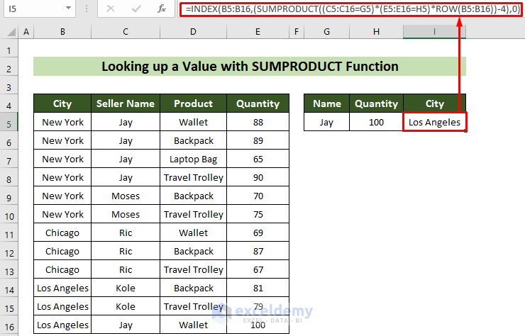
Formula Breakdown:
=SUMPRODUCT((C5:C16=G5)*(E5:E16=H5)*ROW(B5:B16))-4
This returns the row number when the Seller’s name is Jay and the quantity is 100 and subtracts 4.
Result: 12
=INDEX(B5:B16,(SUMPRODUCT((C5:C16=G5)*(E5:E16=H5)*ROW(B5:B16))-4),0)
This returns the value for the previous resultant row of the B5:B16 range.
Result: Los Angeles
- Press Enter.
As a result, you will see the result for Jay in New York with a quantity of 88.
Read More: How to Use SUMPRODUCT IF in Excel
The LOOKUP Function: A Better Alternative to SUMPRODUCT Function to Look Up a Value with Multiple Criteria
Steps:
- Insert your desired criteria in cells G5 and H5.
- Click on cell I5 and insert the following formula:
=LOOKUP(2,1/(C5:C16=G5)/(E5:E16=H5),B5:B16)- Press Enter.
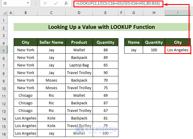
As a result, you can get the desired results in Los Angeles.
Read More: Excel SUMPRODUCT with Multiple Criteria in Same Column
Download the Practice Workbook
You can download our practice workbook from here.
Related Articles
- SUMPRODUCT Across Multiple Sheets in Excel
- SUMPRODUCT for Counting with Multiple Criteria in Excel
- [Solved] SUMPRODUCT with Multiple Criteria Not Working in Excel
<< Go Back to Excel SUMPRODUCT Function | Excel Functions | Learn Excel
Get FREE Advanced Excel Exercises with Solutions!
