How to Use the SUMPRODUCT IF in Excel (2 Methods)

Method 1 – Applying the SUMPRODUCT IF Formula with One Criteria

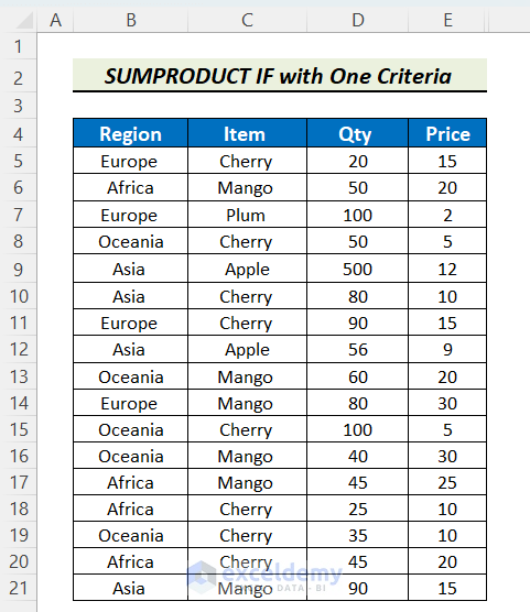
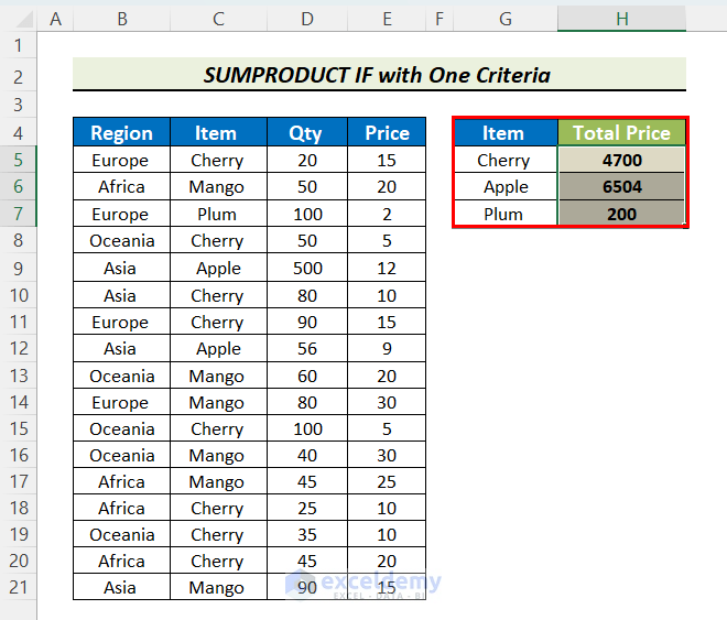
We have a data table with some fruit Items given with “Region,” “Qty,” and “Price.” We will find out the total price of some items.

Steps:

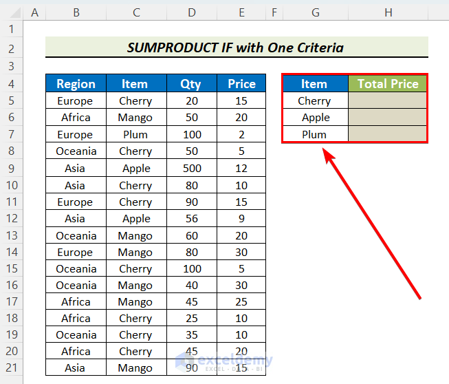
Create another table anywhere on the worksheet where you want to get the total price of the item. We chose “Cherry,” “Apple,” and “Plum” items.

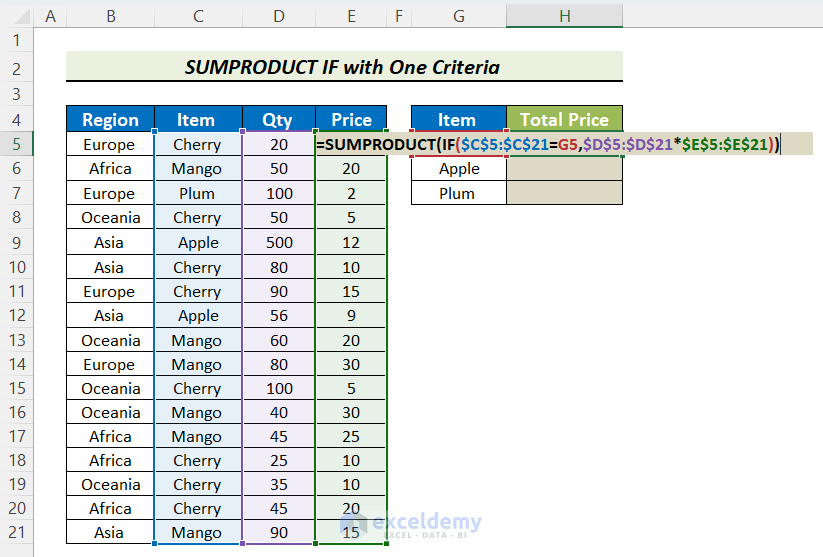
Enter the following formula in cell H4:

=SUMPRODUCT(IF(criteria range=criteria, values range1*values range2))

Enter the values into the formula.

=SUMPRODUCT(IF($C$5:$C$21=G5,$D$5:$D$21*$E$5:$E$21))

Where,

Criteria_range is $C$5:$C$21.
The Criteria are G5, G6 and G7.
Values_range1 is $D$5:$D$21.
Values_range2 is $E$5:$E$21.

Enter this formula as an array formula,
Press CTRL+SHIFT+ENTER. If you are using Excel 365, you can press just ENTER to apply an array formula.

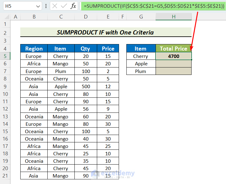
We got our total price. Now apply the same formula for the rest of the items.

Method 2 – Applying the SUMPRODUCT IF Formula with Multiple Criteria in Different Columns

We will use the same formula for multiple criteria.

Steps:

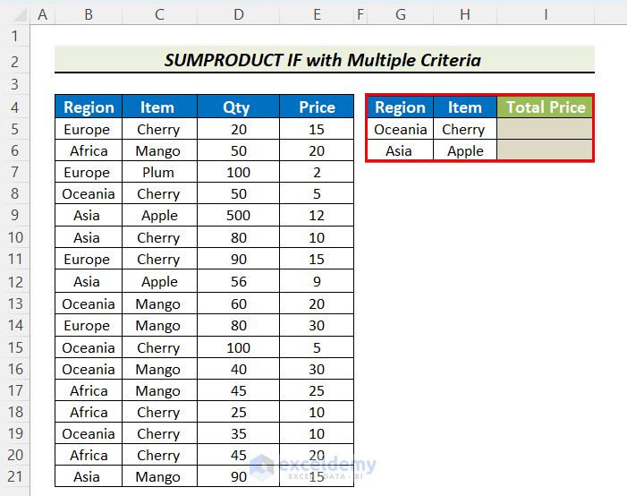
Add another criterion, “Region” in Table 2. We want to find the total price of “Cherry” from the “Oceania” region and “Apple” from the “Asia” region.

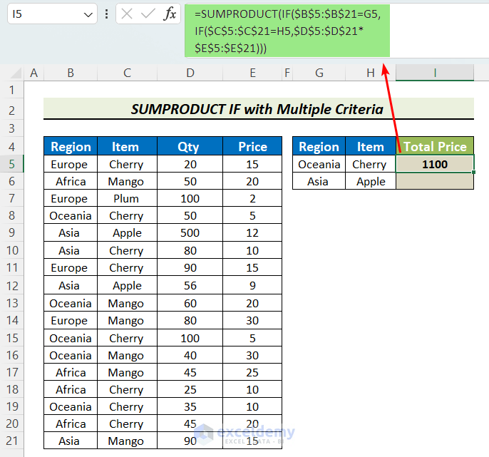
Enter the formula below. Insert the values into the formula.

=SUMPRODUCT(IF($B$5:$B$21=G5,IF($C$5:$C$21=H5,$D$5:$D$21*$E$5:$E$21)))

Where,

Criteria_range is $B$5:$B$21, $C$5:$C$21.
The Criteria is G5, H5.
Values_range1 is $D$5:$D$21.
Values_range2 is $E$5:$E$21.

Press ENTER.

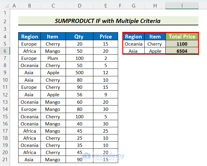
Our value is here. Now do the same for the “Apple” item.

How to Use the ‘Only SUMPRODUCT’ Instead of the SUMPRODUCT IF Formula

There are some other approaches to deriving the previous results. An alternative way to insert the criteria within the SUMPRODUCT function as an array using double unary (–) to convert the TRUE or FALSE into 1 or 0.

SUMPRODUCT with One Condition:

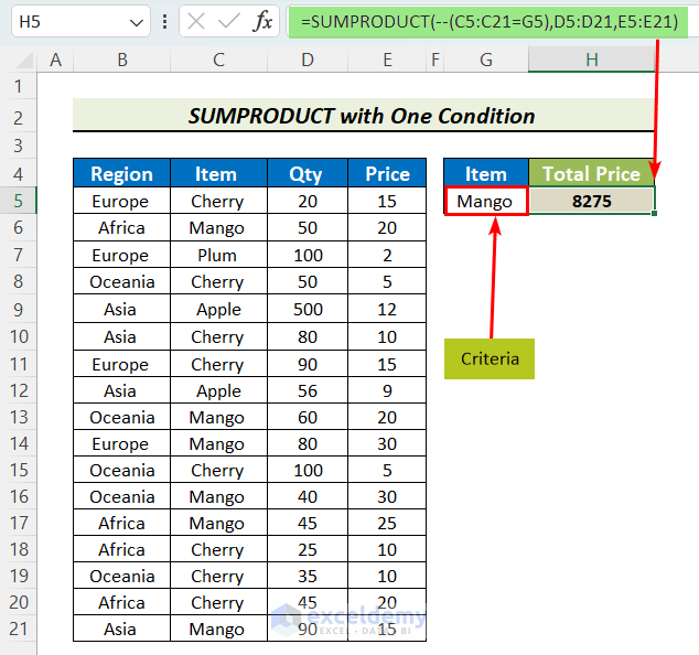
In this case, we will consider the previous example and find the total price of “Mango” from the list.

Apply the conditional SUMPRODUCT formula below.

=SUMPRODUCT(--(C5:C21=G5),D5:D21,E5:E21)

Where,

Array1 is (–(C5:C21=G5).
[Array2] is D5:D21.
[Array3] is E5:E21.

Press “Enter”. Our result is here.

Formula Explanation:

We will now explain how this conditional SUMPRODUCT function works

When we enter the “–(C4:C20=G4)” into the formula, this double unary (–) converts the TRUE or FALSE into 1 or 0. Select this “–(C4:C20=G4)” portion in your worksheet and press “F9” to see the underlying values.
Output: {0,1,0,0,0,0,0,0,1,1,0,1,1,0,0,0,1}

Now if we break down the arrays into values, the actual formula will look like this,

=SUMPRODUCT({0,1,0,0,0,0,0,0,1,1,0,1,1,0,0,0,1},{20,50,100,50,500,80,90,56,60,80,100,40,45,25,35,45,90},{15,20,2,5,12,10,15,9,20,30,5,30,25,10,10,20,15})

The first array will multiply with the second then the second array will multiply with the third array. Follow this picture

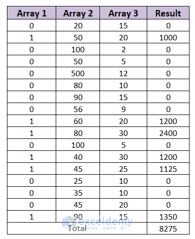
That is how this conditional SUMPRODUCT works.

Applying Multiple Conditions in Different Columns

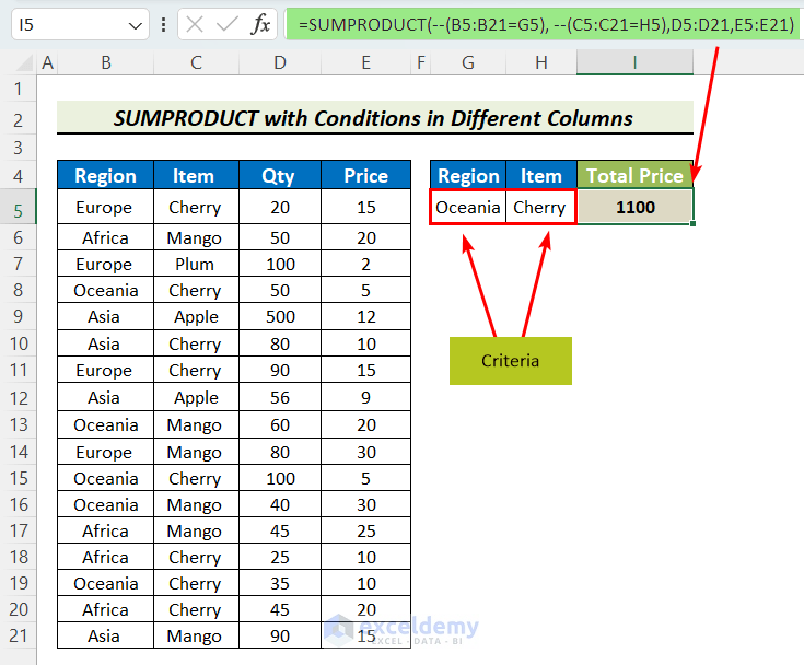
In the following example, we will find the total price of “Cherry” from the “Oceania” region.

Enter the following formula:

=SUMPRODUCT(--(B5:B21=G5), --(C5:C21=H5),D5:D21,E5:E21)

Where,

Array1 is (–(C5:C21=G5),–(C5:C21=H5).
[Array2] is D5:D21.
[Array3] is E5:E21.

Press ENTER. Our result is achieved.

Applying OR Logic

We can add OR logic to our formula to make this formula more dynamic.

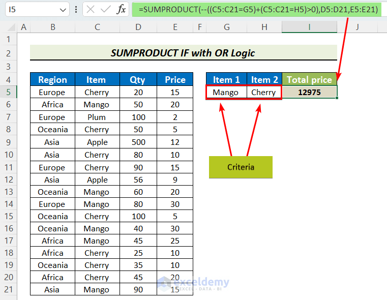
We need to get the total price of “Mango” and “Cherry” from the data table.

Enter the SUMPRODUCT formula with OR and insert the values:

=SUMPRODUCT(--((C5:C21=G5)+(C5:C21=H5)>0),D5:D21,E5:E21)

Where,

Array1 is –((C5:C21=G5)+(C5:C21=H5)>0). Here G5 is “Mango” and H5 is “Cherry”. This array counts the total number of “Mango” and “Cherry” in the data table.
[Array2] is D5:D21.
[Array3] is E5:E21.

Press “Enter” to get the total price of the products.

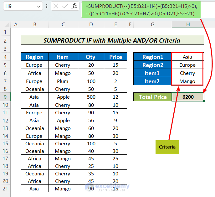
Applying Multiple AND/OR Criteria

We will apply Or logic with multiple conditions.

In the following example, we need to find the total price of “Cherry” and “Mango” from “Asia” and “Europe” regions.

To get the result, we will now apply the formula with AND/OR logic. The formula is

=SUMPRODUCT(--((B5:B21=H4)+(B5:B21=H5)>0),--((C5:C21=H6)+(C5:C21=H7)>0),D5:D21,E5:E21)

Where,

Array1 is –((B5:B21=H4)+(B5:B21=H5)>0),–((C5:C21=H6)+(C5:C21=H7)>0). Here B5:B21 is “Region” Column, H4 and H5 is “Asia” and “Europe”.Similarly,C5:C21 is “Item” column, H6 and H7 is “Cherry” and “Mango”.
[Array2] is D5:D21.
[Array3] is E5:E21.