Excel SUMPRODUCT Function: Overview
Technically, the “SUMPRODUCT” function remits the summation of the values of corresponding arrays or ranges.
⇒ Syntax
The syntax of the “SUMPRODUCT” function is simple and direct.
=SUMPRODUCT(array1, [array2], [array3], …)
⇒ Argument
| Argument | Required/Optional | Explanation |
|---|---|---|
| array1 | Required | The first input to an array, whose elements you want to divide and afterward add. |
| [array2], [array3] | Optional | Array parameters with elements you want to multiply and add, ranging from 2 to 255. |
Note: One of the amazing features of the SUMPRODUCT function is it can handle single or multiple criteria remarkably well. Let’s discuss some of the SUMPRODUCT with criteria functions.
Method 1 – Applying SUMPRODUCT with a Single Criterion to Lookup Value
Case 1.1 – Using Double Unary Operator
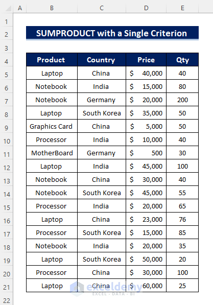
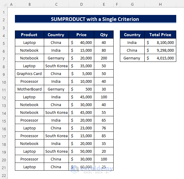
Some Product names are given with their Country, Qty, and Price. We will find the total price for India, China, and Germany.
Steps:
- Create a table for these countries anywhere in the worksheet where you want to get the result.
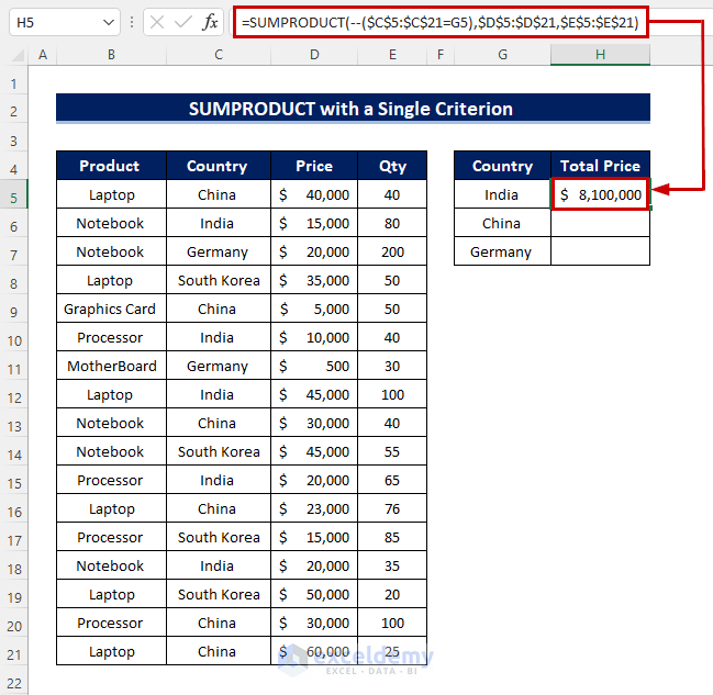
- Select the cell where you want to put the formula of the SUMPRODUCT function.
- Insert the following formula into that cell.
=SUMPRODUCT(--($C$5:$C$21=G5),$D$5:$D$21,$E$5:$E$21)- Press the Enter key.
- Drag the Fill Handle icon down to duplicate the formula over the range or double-click on the plus (+) symbol.
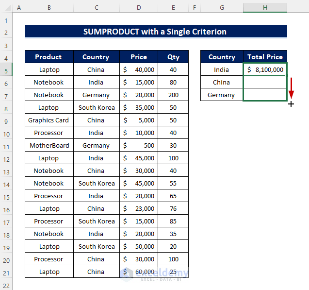
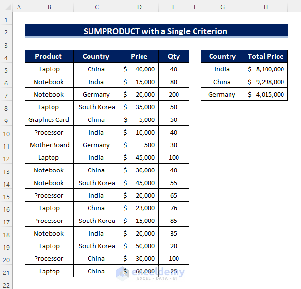
- We can see the results for India, China, and Germany.
How Does the Formula Work?
- Array1 is –($C$5:$C$21=G5) G5 is “India”. The double unary operator will convert the results from $C$4:$C$20 into “1” and “0”.
- [Array2] is $D$5:$D$21, which range we first multiply and then add.
- [Array3] is $E$5:$E$21, also this range we multiply and then add.
Read More: How to Use SUMPRODUCT Function with Multiple Columns in Excel
Case 1.2 – Excluding Double Unary Operator
Steps:
- In Cell H5, apply the following formula:
=SUMPRODUCT(($C$5:$C$21=G5)*$D$5:$D$21*$E$5:$E$21)
- Hit Enter.
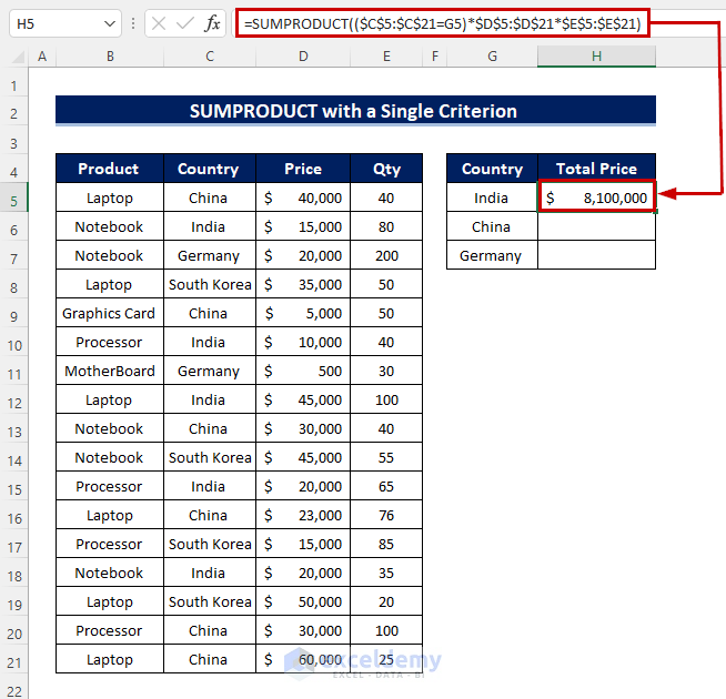
- Drag the Fill Handle symbol down or double-click it to AutoFill the range.
- Here’s the result.
Method 2 – Using SUMPRODUCT with Multiple Criteria for Different Columns
Case 2.1 – Using Double Unary Operator
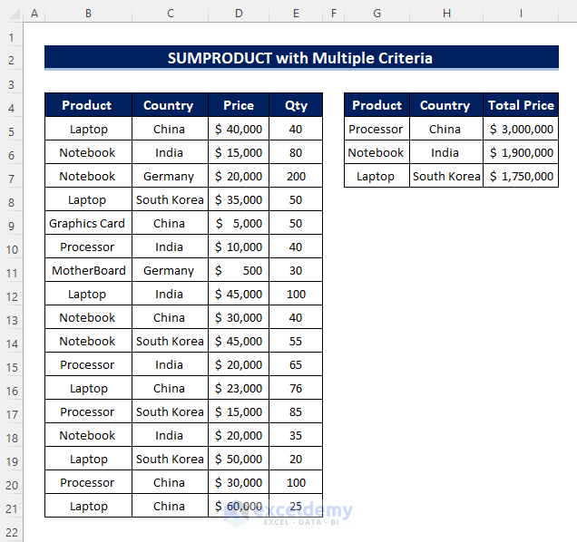
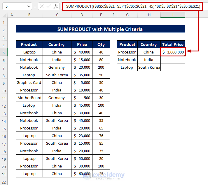
We will find the Total Price for Processor from China, Notebook from India, and Laptop from South Korea.
Steps:
- Select a cell for the first result and enter the following formula.
=SUMPRODUCT(--($B$5:$B$21=G5),--($C$5:$C$21=H5),$D$5:$D$21,$E$5:$E$21)- Press the Enter key.
- Drag the Fill Handle icon down to duplicate the formula over the range or double-click on it.
- You will get the results.
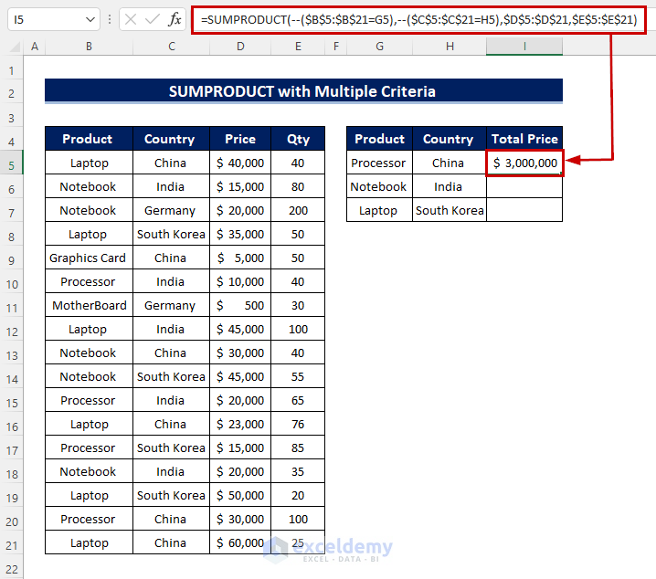
Case 2.2 – Excluding Double Unary Operator
STEPS:
- In cell I5, apply the following function.
=SUMPRODUCT(($B$5:$B$21=G5)*($C$5:$C$21=H5)*$D$5:$D$21*$E$5:$E$21)- Hit Enter to see the result.
- AutoFill through the column.

Read More: How to Use SUMPRODUCT to Lookup Multiple Criteria in Excel
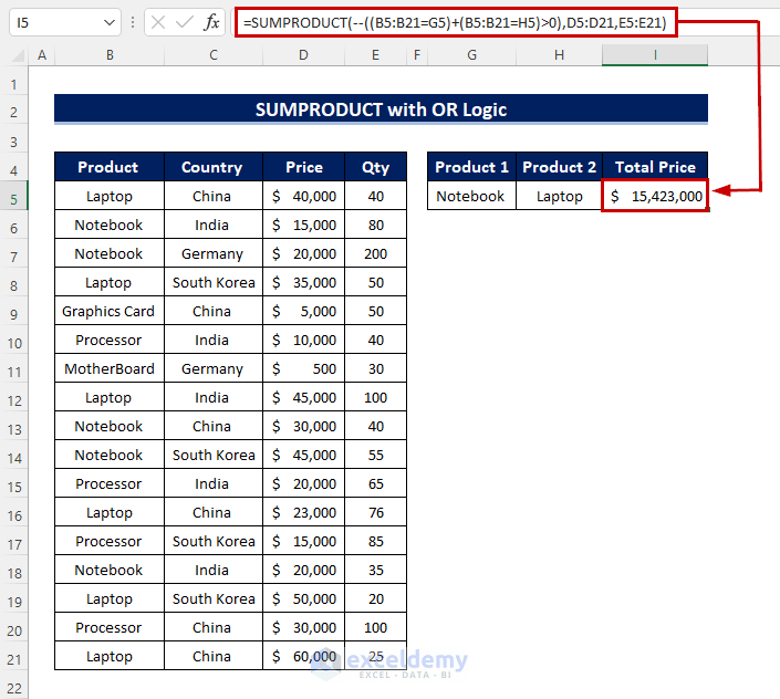
Method 3 – Inserting the SUMPRODUCT Function with OR Logic
We need to find the total price for Notebook and Laptop.
STEPS:
- Create a table anywhere in the worksheet where you want to get the result. List the criteria in two cells in the same row.
- Select the cell and insert the following formula there.
=SUMPRODUCT(--((B5:B21=G5)+(B5:B21=H5)>0),D5:D21,E5:E21)- Hit the Enter key to see the outcome.
Related Content: Excel SUMPRODUCT Function Based on Date Range
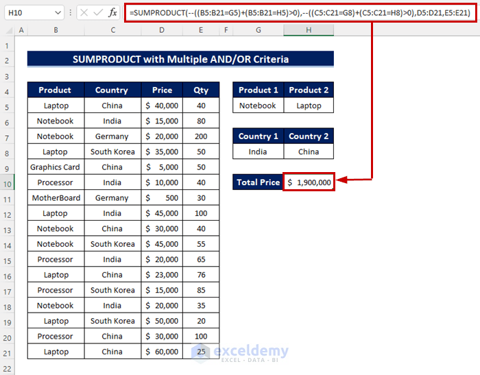
Method 4 – Applying SUMPRODUCT with Multiple AND/OR Criteria
We will retrieve the Total Price for the products Notebook and Laptop from India and China.
STEPS:
- See the image below for creating the criteria cells.
- Select the cell H10 and put the following formula into it.
=SUMPRODUCT(--((B5:B21=G5)+(B5:B21=H5)>0),--((C5:C21=G8)+(C5:C21=H8)>0),D5:D21,E5:E21)- Press the Enter key to see the outcome.
How Does the Formula Work?
- 1 is –((B5:B21=G5)+(B5:B21=H5)>0),–((C5:C21=G8)+(C5:C21=H8)>0). Here B5:B21 is the “Product” Column, G5 and H5 are “Notebook” and “Laptop”. Similarly, C5:C21 is the “Country” column, and G6 and H6 are “India” and “China”.
- [Array2] is D5:D21.
- [Array3] is E5:E21.
Read More: How to Use SUMPRODUCT IF in Excel
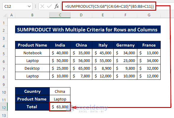
Method 5 – Using SUMPRODUCT with Multiple Criteria for Rows and Columns
We’ll the price of some Products from various countries.
STEPS:
- See image below for a list of criteria.
- Select the cell where we want to put the result.
- Insert the formula into that cell.
=SUMPRODUCT(C5:G8*(C4:G4=C10)*(B5:B8=C11))- Press Enter.
Read More: Excel SUMPRODUCT with Multiple Criteria in Same Column
Things to Remember
✅ The “SUMPRODUCT” function treats non-numeric values as zeros. If you have any non-numeric values in your formula the answer will be “0”.
✅ Arrays in the SUMPRODUCT formula must have the same number of rows and columns. If not, you get the #VALUE! Error.
✅ The “SUMPRODUCT” function does not support wildcard characters.
Download the Practice Workbook
Related Articles
- SUMPRODUCT Across Multiple Sheets in Excel
- SUMPRODUCT for Counting with Multiple Criteria in Excel
- [Solved] SUMPRODUCT with Multiple Criteria Not Working in Excel
<< Go Back to Excel SUMPRODUCT Function | Excel Functions | Learn Excel
Get FREE Advanced Excel Exercises with Solutions!

I believe there’s an error in “5) SUMPRODUCT with Multiple Criteria for Rows and Columns “: the answer calcualated by SUMPRODUCT()($63,800) should actually be only $56,000 (the intersection of Laptop and China).
Dear FLEET,
Thank you for your response.
The answer for the intersection of “Laptop” and “China” will be “$63,800”.
The SUMPRODUCT function returns the sum of an array from an argument. With the intersection between “China” and Laptop” within the cell range we got two outputs which are “$56,000” and “$7,800”. Thus summing the total value with the SUMPRODUCT function stands to “$63,800”.
You can check the screenshot below.
We have also attached a worksheet with our article. You can practice the formula there, too. Thanks!
Thanks for referring, I will check.
u made my day. i was struggling with multiple selections!… thanks a lot
Hello, KRISHNAN V! Thanks for your feedback. Hope you’ll find our other articles useful as well when needed for your works!
How can I use the SUMPRODUCT for adding sums from different columns that are under the same category in a drop-down list? For this example, I split up my expenses for each pay check and then I categorize each expense by an “expense type”. I want each expense for each expense type to be added together to a separate table that I will then use those sums to create a pie chart. For example, I have a pay check on 9/15 where my Lifestyle expense = $200 and a pay check on 9/30 where the Lifestyle expense= $350. In the other table, I want to be able to add the sum of $200+$350. Can SUMPRODUCT help me with this? I have been struggling a lot to figure this out! I can provide a screen shot of the excel chart if needed.
Hello FELICIA SANTOS,
I hope you are doing well! Here, I have created a dataset as you have described and calculated the total amount spent per category.
>> Here, you have to insert the name of the category in cell F5.
>> Then, insert the following formula into cell G5:
=SUMPRODUCT(D3:D10*(C3:C10=F5))Thus, you will get the sum of the amount as per the selected category.
I hope, your problem will be solved in this way. You can share more problems in an email at [email protected]
Hi,
What if I want to sum Notebook from India up to France (Result = $ 167,000.00)
or
Product : Notebook
From : China
To : Germany
Result = $114,000
From & To in dropdown list
Hello DRIN,
Thanks for your comment.
If you want to sum Notebook from India up to France and use drop-down for the countries, then use the following formula in cell C13:
=SUM(INDEX($B$5:$G$8,MATCH(C10,$B$5:$B$8,0),MATCH(C11,$C$4:$G$4,0)+1):INDEX($B$5:$G$8,MATCH(C10,$B$5:$B$8,0),MATCH(C12,$C$4:$G$4,0)+1))
It’ll give the desired result.
Change the countries to China and Germany from the drop-down and the total value will be updated.
If you have other queries let me know in the comment.
Regards,
Sajid Ahmed
Exceldemy
very help information. I managed to resolve my equation for sumproduct.
Thanks a lot
KS
Hello,
You are most welcome.
Regards
ExcelDemy