Microsoft Excel offers a variety of methods for counting multiple conditions. We may do this by filtering data using PivotTable or the COUNTIF function. Although hardly any of those methods offer the SUMPRODUCT function’s level of adaptability. In this article, we will demonstrate some examples to use the SUMPRODUCT function for counting with multiple criteria in Excel.
Introduction to Excel SUMPRODUCT Function
One or more arrays can be sent as arguments to SUMPRODUCT, which multiplies the corresponding values of each array before returning the sum of the products.
⇒ Syntax
The syntax of the SUMPRODUCT function is:
SUMPRODUCT(array1,[array2],[array3],…)
⇒ Argument
array1: (Required) The first array of numbers.
array2: (Optional) The second array of numbers.
array3: (Optional) The third array of numbers.
⇒ Return Value
Returns the sum of the products of the corresponding values from all the arrays.
Read More: How to Use SUMPRODUCT with Criteria in Excel
SUMPRODUCT for Counting with Multiple Criteria in Excel: 3 Ideal Examples
The SUMPRODUCT function in Excel could be able to help you if you need to count a range depending on a variety of criteria, some of the criteria are dependent on the logical tests. Let’s look at the examples of using this function for counting with multiple criteria.
1. Count Rows with Multiple Criteria Using Excel SUMPRODUCT Function
Counting rows that satisfy several criteria by utilizing Excel’s SUMPRODUCT function, we need to follow the procedures down.
STEPS:
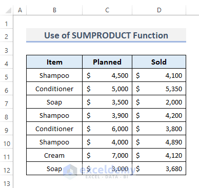
- Firstly, we have to set up the dataset. For instance, we have a dataset that contains some items, the assumed amount of sales money which we name the column planned for, and also the original number of sales.
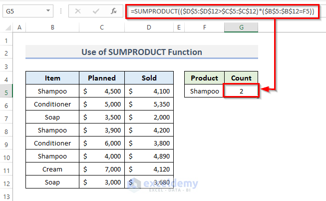
- Secondly, select the cell G5 where we want to determine how many Shampoo rows really sold more than was planned.
=SUMPRODUCT(($D$5:$D$12>$C$5:$C$12)*($B$5:$B$12=F5))- Then, press the Enter key to obtain the desired outcome.
🔎 How Does the Formula Work?
- $D$5:$D$12>$C$5:$C$12: The values of each row’s columns D and C are contrasted using this logical formula. A TRUE message appears if the D column’s value exceeds column C‘s value. If not, a FALSE will appear and the array values will be returned as follows: FALSE;TRUE;FALSE;TRUE;FALSE;TRUE;FALSE;TRUE.
- $B$5:$B$12=F5: This logical statement determines if cell F5 is present in the range B5:B10. As a consequence, you will receive the following result:
TRUE;FALSE;FALSE;TRUE;FALSE;TRUE;FALSE;FALSE. - ($D$5:$D$12>$C$5:$C$12)*($B$5:$B$12=F5): These two arrays are multiplied into a single array using the multiplication operation, which yields the following result: 0;0;0;1;0;1;0;0.
- SUMPRODUCT(($D$5:$D$12>$C$5:$C$12)*($B$5:$B$12=F5)): This SUMPRODUCT totals the integers in the array and outputs the following result: 2.
Read More: How to Use SUMPRODUCT Function with Multiple Columns in Excel
2. Apply SUMPRODUCT for Counting Consumers Based on Multiple Criteria
In this example, we will look at the multiple OR criteria with the SUMPRODUCT function. The plus sign (+) would be used if OR logic were necessary. For this, let’s follow the steps below.
STEPS:
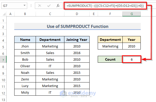
- In the first place, we just need a dataset. Suppose, we have some employees, their departments, and the joining year. Now we need to determine how many people have the ‘Marketing’ department or the joining year ‘2010’. Make sure that if a person has both the year 2010 and the department ‘Marketing’, count them as 1.

- Next, choose the cell where the formula should go. Here, it is G7.
=SUMPRODUCT(--(((C5:C12=F5)+(D5:D12=G5))>0))- Then, to get the result you want, press the Enter key.
🔎 How Does the Formula Work?
- C5:C12=F5: This is for the comparison, if the condition is met it will return TRUE otherwise FALSE. The value of the array is: TRUE;FALSE;FALSE;FALSE;FALSE;TRUE;TRUE; FALSE.
- D5:D12=G5: The outcome will be as follows: TRUE;FALSE;TRUE;FALSE;FALSE;TRUE;FALSE;TRUE.
- (C5:C12=F5)+(D5:D12=G5): The array produces the outcome seen below: 2;0;1;1;0;2;1;1.
- SUMPRODUCT(–(((C5:C12=F5)+(D5:D12=G5))>0)): This results in the following: 6.
Related Content: Excel SUMPRODUCT Function Based on Date Range
3. Count with Multiple Conditions Using the SUMPRODUCT Function
This example will show the counting with multiple conditions using the Excel SUMPRODUCT function. Applying AND logic between each condition is done using the multiplication operator (*). Follow the instructions to use the SUMPRODUCT function for counting with multiple criteria.
STEPS:
- To begin with, create a dataset. The dataset accommodates some dates, items, customers, and sales. Now, we need to count the number of orders if this fulfills the conditions.

- Select the cell (H6) where the formula should go next.
=SUMPRODUCT((C5:C12=H4)*(D5:D12=H5))- Finally, hit Enter to get the result you want.

🔎 How Does the Formula Work?
- C5:C12=H4): You’ll get the following outcome: TRUE;FALSE;FALSE;TRUE;TRUE;FALSE;FALSE;FALSE.
- D5:D12=H5: It produces the following outcome: TRUE;FALSE;TRUE;FALSE;TRUE;FALSE;TRUE;FALSE.
- SUMPRODUCT((C5:C12=H4)*(D5:D12=H5)): The array generates the following outcome: 2.
Read More: How to Use SUMPRODUCT IF in Excel
Things to Keep in Mind
- Although it uses arrays, the formula is non-array. To insert this function, you do not need to use Ctrl + Shift + Enter.
- Each array’s length must be the same. Excel will issue a #VALUE! error otherwise.
- The arrays used by the SUMPRODUCT function typically include all integers. However, SUMPRODUCT will treat every cell in an array that has a text value rather than a number as zero.
- You may put a ‘–’ in front of an array to make it into an array of integers if it only includes Boolean values (TRUE and FALSE). 0 for FALSE, 1 for TRUE.
Download Practice Workbook
You can download the workbook and practice with them.
Conclusion
The above examples will assist you in using the SUMPRODUCT Function for Counting with Multiple Criteria in Excel. Hope this will help you! Please let us know in the comment section if you have any questions, suggestions, or feedback.
Related Articles
- SUMPRODUCT Across Multiple Sheets in Excel
- [Solved] SUMPRODUCT with Multiple Criteria Not Working in Excel
- How to Use SUMPRODUCT to Lookup Multiple Criteria in Excel
- Excel SUMPRODUCT with Multiple Criteria in Same Column
<< Go Back to Excel SUMPRODUCT Function | Excel Functions | Learn Excel
Get FREE Advanced Excel Exercises with Solutions!
