Latest Posts From Sabrina Ayon

Method 1 - Apply an Excel VBA Code for a HTML Decode String Steps: Go to the Developer tab from the ribbon. Click on Visual Basic ...

Method 1 - Utilize Data Labels of Excel Graph to Convert Decimal Places STEPS: Insert the graph. For this, select the data. Go to the Insert tab from ...
![[Fixed] Excel Data Table Input Cell Reference Is Not Valid](https://www.exceldemy.com/wp-content/uploads/2022/11/excel-data-table-input-cell-reference-is-not-valid-1-1.png?v=1697439878)
Reason 1 - Input Cell Is in Different Sheet An input cell reference is not valid error message could appear when using a data table where input cell makes a ...
Step 1 - Launch the Excel Developer Tab If you have the Developer tab on your ribbon, you can skip this step. Right-click on the ribbon and go to ...
Method 1 - Utilize Excel Ribbon to Generate Excel Form STEPS: Go to the Page Layout tab from the ribbon. Click on the Size drop-down menu ...
You have a blank PPT file saved in Drive (D:). Step 1 - Launch the Developer Tab Right-click the ribbon. Select Customize the Ribbon. ...
![[Fixed] Excel Macros Enabled But Not Working](https://www.exceldemy.com/wp-content/uploads/2022/11/macros-enabled-but-not-working-9.png?v=1697440255)
Reason 1 - Worksheet Might Be Saved as an .xlsx File The file extension for spreadsheets that support macros is .xlsm, whereas that of unmodified ...
Method 1 - Summary of TDS for Late Deduction We record all the sections and type in column C and TDS statement for the month of November, December and ...

We may have irregular income, which means that your take-home pay fluctuates from one pay period to another pay period. Our income won't likely be as steady if ...

Let’s look at the ways to move the barcode scanner to the next row in Excel. We'll use a simple dataset with random product codes. Method 1 - ...
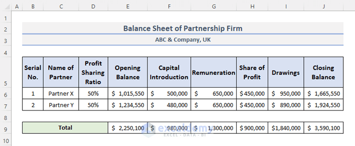
Step 1 - Make an Excel Document Prepare the Excel file to create a format of the balance sheet of the partnership firm. We put two headings; one is the ...

Method 1 - Using the AVERAGEIF Function in Excel STEPS: We need to create a dataset. We have some students' names and their marks for a subject. We want ...

Microsoft Excel offers a variety of methods for counting multiple conditions. We may do this by filtering data using PivotTable or the COUNTIF function. ...
Method 1 - Utilizing Format Cells Feature to Prevent Excel from Converting Numbers to Dates The format cells feature allows us to change the appearance of ...
If we have the addresses of two specific cities or locations on the planet, we can calculate the travel time between them in Excel by making use of a third ...
- 1
- 2
- 3
- …
- 10
- Next Page »
See Our Reviews at


Hello, E!
Did you follow those steps properly? If any of those did not work, then try this out!
Sub Inert_rows()
Dim rng As Long
For rng = range(“C” & Rows.Count).End(xlUp).Row To 1 Step -1
With Cells(rng, 3)
If IsNumeric(.Value) And Not IsEmpty(.Value) Then
Rows(rng + 1).Resize(.Value).Insert
range(Replace(“G#:BW#”, “#”, rng)).Copy Destination:=range(“G” & rng + 1).Resize(.Value)
End If
End With
Next rng
End Sub
Hello, HUNTER!
Thanks for sharing your problem with us!
To add a condition in the code from step 1 to only send once a day, you can use a global variable to keep track of the last time an email was sent. Here’s an example of how you can modify the code:
In this modified code, the lastSentTime variable is used to keep track of the last time an email was sent. When a cell is changed and meets the criteria for sending an email, the code checks if at least one day has passed since the last email was sent before sending a new email. If less than a day has passed, the code skips sending the email. Once an email is sent, the lastSentTime variable is updated with the current time.
Hope this will help you.
Good Luck!
Regards,
Sabrina Ayon
Author, ExcelDemy.
Hello, JOHN!
Thanks for your comment!
I’m not sure about your problem, you want all Lenovos that means the Desktop and Notebook! Also, All the desktops that mean the range of C5:C9!
Can you please send me your excel file via email? ([email protected]).
You can use this https://www.exceldemy.com/sum-index-match-multiple-criteria-in-excel/#Use_of_SUMIFS_with_INDEX_MATCH_Functions_in_Excel
This may fulfill your criteria.
Good Luck!
Regards,
Sabrina Ayon
Author, ExcelDemy.
Hello, AMIR!
Thanks for your comment.
Yes! The code you provided is a simple implementation for converting latitude and longitude to UTM in Excel VBA. However, it is not the most accurate way to convert coordinates, as it uses a simplified formula for converting latitude and longitude to UTM coordinates.
The formula used in this code only accounts for the UTM zone and hemisphere based on the latitude and longitude values. It does not take into account the curvature of the Earth’s surface, which can lead to inaccuracies in the UTM coordinates. If you need this, then you can use the following code:
To use this code, open a new Excel workbook, press ALT+F11 to open the VBA editor, and insert a new module. Copy and paste the code into the module, and save the module.
Then, in your Excel sheet, you can use the formula =LatLonToUTM(lat, lon) where lat and lon are the latitude and longitude coordinates you want to convert to UTM format.
This code uses the Proj4 library to perform the coordinate transformation. You may need to install this library on your computer if it is not already installed.
And if you don’t want to use this library. you can use the following code instead.
This code converts latitude and longitude coordinates to UTM coordinates and returns the result as a string in the format "Zone Letter X Y". You can call this function by passing the latitude and longitude values as parameters, like this:
Make sure you have the LatLongToUTM function defined in your VBA code module before running the ConvertLatLongToUTM sub.
Hope this will help you.
Good Luck!
Regards,
Sabrina Ayon
Author, ExcelDemy.
Hello, OBOT!
Thanks for your comment!
To import data from a specific sheet (e.g., “Sheet2“) of a Google Sheets document to Excel using VBA, you can use the following code:
To use this code, you need to replace the googleSheetsURL variable with the URL of the Google Sheets document containing the data you want to import and replace the sheetName variable with the name of the sheet containing the data you want to import (in this example, “Sheet2“). You also need to set the targetRange variable to specify the cell or range where you want to paste the imported data (in this example, cell A1 of the Sheet1 worksheet).
The code uses the MSXML2.XMLHTTP object to send an HTTP request to the Google Sheets document, and parses the HTML response to identify the range of cells corresponding to the specified sheet name. It then copies the data from the identified range to the clipboard, clears the target range to ensure that no existing data interferes with the import, and pastes the data from the clipboard into the target range.
Hope this will help you!
Good Luck!
Regards,
Sabrina Ayon
Author, ExcelDemy.
Hello, MRS B!
Can you please send me your excel file via email? ([email protected]), so that I can solve your problem!
Right now I’m giving you a quick solution without the dataset. You can use Excel’s VLOOKUP function to have fields in the payment request form automatically fill in depending on the employee number.
Here is a formula that uses the VLOOKUP function as an example:
=VLOOKUP(employee number,employee table,2,FALSE)Here, “Employee number” refers to the cell where the employee number input is located, “Employee table” refers to the cell range containing the employee information table, which includes the employee number in the first column, and “2” refers to the column number in the table that contains the university information.
You can change this formula to return different data. Once the relevant information has been obtained from the table, you can use it to fill in the essential fields on the payment request form by utilizing straightforward cell references or other procedures.
Hope this will help you.
Good Luck!
Regards,
Sabrina Ayon
Author, ExcelDemy.
Hello, UDAY KUMAR!
It seems that the error message you received is related to the use of reference operators in the formula.
The formula you were using in the conditional formatting rule contains a reference operator and the INDEX function, which can be interpreted as an array constant. The error message you received indicates that the use of such operators and array constants is not allowed in conditional formatting criteria.
To avoid using the reference operator and array constant, you can use the INDIRECT function. Here’s an example formula that uses the INDIRECT function:
=SUM(INDIRECT("B$3:B" & ROW()))<=$B$35The INDIRECT function takes a text string argument that specifies a cell reference and returns the value of the cell. By concatenating the starting and ending cell references with the ROW function, we can create a dynamic reference to the range we want to sum.
Hope this will help you. If not, can you please send me your excel file via email? ([email protected]).
Good Luck!
Regards,
Sabrina Ayon
Author, ExcelDemy.
Hello, EHTISHAM SAFDAR!
Thanks a ton for your suggestion!
In Method-7, the precise range we require to count the number of cells containing dates is D5:D12. Determines whether each data value in a given array or range is legitimate by SUM each one.
Regards,
Sabrina Ayon
Author, ExcelDemy.
Hello, BILL SHIELDS!
Thanks for your appreciation!
Stay connected with Exceldemy.
Good Luck!
Regards,
Sabrina Ayon
Author, ExcelDemy.
Hello, OZTIMS!
Thanks for sharing your problem with us!
Instead of using this format ($General;;), you can use the ($0;-0;;@). This will keep the negative values. To use this follow method-4.
1. When the Format Cells dialog box will appear, go to Number > Custom.
2. Type $0;-0;;@ in the Type field.
3. Finally, click OK.
4. Now, if you see the result, this will also show a negative number. The cell will only be blank if the cell has no data.
Hope this will help you.
Good Luck!
Regards,
Sabrina Ayon
Author, ExcelDemy.
Hello, Billy!
Thanks for sharing your problem with us!
Actually, this code perfectly works for me. This code extracts specific data from pdf to Excel properly. Please, make sure you use the accurate Application and PDF paths.
Can you please send me your excel file via email? ([email protected]).
So that, I can solve your problem.
Good Luck!
Regards,
Sabrina Ayon
Author, ExcelDemy.
Hello, DONI!
Thanks for sharing your problem with us!
All the methods work properly for me. I am also using Microsoft Office 365.
Can you please send me your excel file via email? ([email protected]).
So that, I can solve your problem.
Good Luck!
Regards,
Sabrina Ayon
Author, ExcelDemy.
Hello, Bob!
Thanks for your comment!
Yes! This formula won’t work in Excel 2016. I will suggest that use Excel 365.
Good Luck!
Regards,
Sabrina Ayon
Author, ExcelDemy.
Hello, JHORDISTA!
Thanks for your comment. To format a negative number showing parenthesis, you can add this block of code with any of the above VBA code.
Hope this will help you!
Good Luck!
Regards,
Sabrina Ayon
Author, ExcelDemy.
Hello, DANIEL DUMITRU!
Thanks for your comment. Appreciate your efforts. Stay connected with us!
Good Luck!
Regards,
Sabrina Ayon
Author, ExcelDemy.
Hello, ASHLEY!
Thanks for your comment.
Yes. Unfortunately, the google charts API is currently broken. You can use the following API which I updated in the article.
https://chart.googleapis.com/chart?chs=100×100&&cht=qr&chl=
Try out this code below.
Hope this will help you!
Good Luck!
Regards,
Sabrina Ayon
Author, ExcelDemy.
Hello, LOCHIA!
Thanks for sharing your problem with us!
Actually, in the following formula, C stands for Column, and R stands for Row. The While loop block of codes is searching Column C in a loop for values that match. Up until there is no match, iteration continues. If no match is found, it tosses the Sum value.
="=SUM(R" & xValue & "C:R" & iValue & "C)"Can you please send me your excel file via email? ([email protected]).
So that, I can solve your problem.
Good Luck!
Regards,
Sabrina Ayon
Author, ExcelDemy.
Hello, AMIRA!
Thanks for sharing your problem with us!
The code works properly for me.
Can you please send me your excel file via email? ([email protected]).
So that, I can solve your problem.
Good Luck!
Regards,
Sabrina Ayon
Author, ExcelDemy.
Thanks, SR DIABLO!
Thanks for your comment!
Yes, you are right! Actually, the purpose of this line is the same as the loop. You can either use this block of code.
Alternatively, you can use this line instead of using the loop.
You can skip the line or comment on the line using an apostrophe in front of the line you wish to turn into non-executable code. It’s actually not a mistake. The code will work properly if you do not remove it! But I suggest you use any one of those.
Good Luck!
Regards,
Sabrina Ayon
Author, ExcelDemy.
Hello, GABRIEL!
Thanks for sharing your problem with us!
To add a new line you don’t have to write the command .Insert. You can simply use this block of the code to breakline in the string before cFnd.
To use vbNewLine, you have to make sure to do the following.
1. After the ampersand (&) symbol, press the spacebar and get the VBA constant ‘vbNewLine‘.
2. After the constant ‘vbNewLine‘, press one more time space bar and add the ampersand (&) symbol.
3. After the second ampersand (&) symbol, type one more space character, and add the next line sentence in double-quotes.
In VBA, there are three different (constants) to add a line break.
vbNewLine, vbCrLf, vbLf
If this is not working for you, follow the steps.
1. Click on the character you wish to break the line from first.
2. Then, enter a space ( ).
3. Type an underscore (_) after that.
4. Finally, press Enter to finish the line.
Hope this will help you!
Good Luck!
Regards,
Sabrina Ayon
Author, ExcelDemy.
Hello, DALE HALL!
Thanks for sharing your problem with us!
You can set a range of cells to highlight using the following VBA code.
Hope this will help you!
Good Luck!
Regards,
Sabrina Ayon
Author, ExcelDemy.
Hello, Rick!
Thanks for sharing your problem with us!
While copying, you have to copy the whole thing (values + formulas). You can have the values (without any formula) only while pasting the copied portion into another place.
While pasting, instead of using ‘.Paste‘ to replicate a formula result as a value rather than the formula itself, use ‘.PasteSpecial‘.
Hope this will help you!
Good Luck!
Regards,
Sabrina Ayon
Author, ExcelDemy.
Hello, Niki!
Thanks for sharing your problem with us!
You can use the formula to find the second last result from a certain cell.
For this,
1. Select the cell where you want to see the result.
2. Insert the formula into the formula bar.
=INDEX(D:D,LARGE(IF(D:D<>"",ROW(D:D)),2))3. Press Shift + Ctrl + Enter.
Note: You have to press Shift + Ctrl + Enter together, otherwise the formula won’t work.
Can you please send me your dataset at ([email protected]), so that I can help you?
Hope this will help you!
Good Luck!
Regards,
Sabrina Ayon
Author, ExcelDemy.
Hello, JOHN!
Thanks for your comment!
You can lock the row after the date auto updates with the following code.
A cell should only be locked if cell A1 was updated and it is not blank, according to this formula: if Target.Address = “$A$1” and Target.Value > “”
Just substitute the relevant cell value for $A$1 to make the macro function on cell B1, cell D15, or any other cell. For this to function, the column and row references must be preceded by dollar signs.
By changing > “” in the line above to = “desired value,” you may additionally lock the cell only if a certain value was entered, allowing you to do things like lock the cell only if OK was entered or anything similar.
Hope this will help you!
Good Luck!
Regards,
Sabrina Ayon
Author, ExcelDemy.
Hello, DWIGHT!
Thanks for your comment.
Yes! You have to update the range manually in the code.
Regards,
Sabrina Ayon
Author, ExcelDemy.
Hello, MAC!
Thanks for sharing your problem with us!
To integrate these 2 codes, all you need to do is just define the first sub-procedure name in the second part of the code and add the sheet name there before the range-bounded combination. “Worksheet_Change Sheet1.Range(“B5”).Validation…….” like this.
The code should look like this.
Hope this will help you!
Good Luck!
Regards,
Sabrina Ayon
Author, ExcelDemy.
Hello, COLE!
Thanks for sharing your problem with us!
Can you please send me your Excel file at [email protected]? So that, I can help you.
Good Luck!
Regards,
Sabrina Ayon
Author, ExcelDemy.
Hello, AUSTIN!
Thanks for sharing your problem with us!
To convert values into timestamps, follow the instructions below.
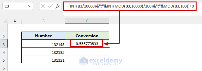
1. select the cell and put the formula into that cell.
2. Press Enter.
=(INT(B3/10000)&":"&INT(MOD(B3,10000)/100)&":"&MOD(B3,100))+03. This will convert the values into time values.
4. Now, go to Home tab by selecting the resulted cell and click on Number Format drop-down menu under Number group.
5. Drag the Fill Handle icon down to duplicate the formula over the range. Or, to AutoFill the range, double-click on the plus (+) symbol.
6. And, that’s it! But there is an issue. as 13 represent 1 in time, so 13 will replaced by 1.
Hope this will help you!
If not, can you please send me your excel file via email? ([email protected]).
Good Luck!
Best Regards
Sabrina Ayon
Author, ExcelDemy.
Hello, LIZ!
Thanks for sharing your problem with us!
Excel automatically detects all difficulties when you interact with it, including inaccurate data in the cell, issues with formulae, etc. As a result, the top left corner of these cells is shown (by default) with green triangles. Excel displays green triangles, this green triangle indicates a potential mistake, although it is frequently ineffective.
Do the following to disable these green triangles or automatic calculation checks:
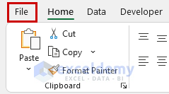
1. Go to the File tab from the ribbon.
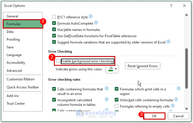
2. Select the Options option from the File tab.
3. Enable background error checking is an option that may be disabled in the Excel Options dialog box’s Formulas tab’s Error Checking section.
All open workbooks in the Excel session will be affected by this application-level option.
Hope this will help you!
If not, can you please send me your excel file via email? ([email protected]).
Good Luck!
Best Regards
Sabrina Ayon
Author, ExcelDemy.
Hello, JAMES RICHMOND!
Thanks for sharing your problem with us!
Please follow the method below. You will find your solution there.
https://www.exceldemy.com/copy-hyperlink-in-excel/#3_Copy_Hyperlink_in_Excel_to_Multiple_Sheets
Good Luck!
Regards,
Sabrina Ayon,
Author, ExcelDemy.
Hello, DANDELION!
Please select the range properly, this macro also works for more than 100 duplicates. There is no limitation. All you need to do is after running the code select the range properly.
Good Luck!
Regards,
Sabrina Ayon
Author, ExcelDemy.
Hello, GIA!
As you mentioned, you fill out Column C with data, and Column B will automatically update with the date when Column C was filled out. All you need to do is change the range in your code, and also change the reference argument which is the offset. Try this code below.
Also, you can use the same code for column E to automatically update with the date and time when you fill Column D with “Delivered”. You just have to change the range.
Please follow the instructions of the method I linked down.
https://www.exceldemy.com/auto-populate-date-in-excel-when-cell-is-updated/#2_Auto_Populate_Dates_in_Some_Specific_Cells_While_Updating_with_Excel_VBA
Hope this will help you!
Best Regards.
Hello, VICKIE WATT!
Thanks for your comment. Yes, this is date static.
You are most welcome, Wayne Edmondson!
Stay Tuned!
Regards,
Sabrina Ayon
Author, ExcelDemy.
Hello, WAYNE EDMONDSON!
Thanks for sharing your thoughts with us!
Stay Tuned!
Regards,
Sabrina Ayon
Author, ExcelDemy.
Hello, HANNES!
You can use the same code to generate 2 screenshots (from 2 different ranges) from the same worksheet. All you have to do is, while selecting any range press Ctrl. Then, just Run the code.
Or, you can use the code below, this will convert your excel file range to word document.
Private Sub EmailSS(rng As Range, rng2 As Range, strName As String)
‘To Open Email
Dim outlookApp As Outlook.Application
Set outlookApp = CreateObject(“Outlook.Application”)
Dim outMail As Outlook.MailItem
Set outMail = outlookApp.CreateItem(olMailItem)
With outMail
.To = strName
.Subject = “** Check this **”
.Importance = olImportanceHigh
.Display
End With
‘To Get Word Document
Dim wordDoc As Word.Document
Set wordDoc = outMail.GetInspector.WordEditor
‘To Take Screenshot
rng.Copy
wordDoc.Paragraphs(1).Range.PasteSpecial , , , , wdPasteBitmap
wordDoc.Content.InsertParagraphAfter
rng2.Copy
wordDoc.Paragraphs(2).Range.PasteSpecial , , , , wdPasteBitmap
outMail.HTMLBody = “Timesheets Submitted by ” & strName & “
” & _
Range(“Text”) & vbNewLine & outMail.HTMLBody
End Sub
Hope this will help you!
Thanks for sharing your problem with use.
Hello, Jim!
Thanks for your comment!
Glad that you noticed!
But it’s not a problem or it’s not even any bug, as I set snam to sf and sf is declared.
I did not set any path where I would put the pdf to print it. That’s the reason I did not set any file path location or declare the strPathFile variable. This code will automatically save into your active disk location. If you want to save the file in a specific file path you can initialize strPathFile and put your path manually.
I will suggest that you please download the workbook and run the codes. After that, if you have any queries you can ask!
Good Luck!
Hello, DEMI!
Please follow step 7, you will surely get the Regions button. If you miss any of those steps you won’t get the result. Follow each instruction step by step hopefully, you will find the Regions button.
https://www.exceldemy.com/create-custom-regions-in-excel-3d-maps/#Step_7_Create_Custom_Regions
Good Luck!
Hello, DJ!
If you just Autofit all the selected rows you can use this code.
Sub Autofit_Rows()
Range(“A1:A10”).Select
Selection.Rows.AutoFit
Range(“A1”).Select
End Sub
After Autofit the rows, double the height of all rows is not possible actually. You can Autofit with some padding, please try this code. Hope this will help you.
Sub AutoFitRows()
Dim ws As Worksheet
Dim rng As Range
Application.ScreenUpdating = False
For Each ws In ActiveWindow.SelectedSheets
With ws.UsedRange
.EntireRow.AutoFit
For Each rng In .Rows
rng.RowHeight = rng.RowHeight + 15
Next rng
.VerticalAlignment = xlCenter
End With
Next ws
Application.ScreenUpdating = True
End Sub
Hello, JAMES!
Those codes work properly for pivot table range. Can you please send me your Excel file at [email protected]? So that, I can help you.
Thanks!
Hello, ROWAN!
Check this article. This may help you.
https://www.exceldemy.com/excel-automatically-send-email-when-condition-met/#2_Send_Email_Automatically_Based_on_a_Due_Date_Using_VBA_Code
Use this code to send 20+ emails in one go each with a unique range. Just change the condition and range as per your requirements.
Public Sub Send_Email_Automatically()
Dim rngD, rngS, rngT As Range
Dim ob1, ob2 As Object
Dim LRow, x As Long
Dim l, strbody, rSendValue, mSub As String
On Error Resume Next
Set rngD = Application.InputBox(“Deadline Range:”, “Exceldemy”, , , , , , 8)
If rngD Is Nothing Then Exit Sub
Set rngS = Application.InputBox(“Email Range:”, “Exceldemy”, , , , , , 8)
If rngS Is Nothing Then Exit Sub
Set rngT = Application.InputBox(“Email Topic Range:”, “Exceldemy”, , , , , , 8)
If rngT Is Nothing Then Exit Sub
LRow = rngD.Rows.Count
Set rngD = rngD(1)
Set rngS = rngS(1)
Set rngT = rngT(1)
Set ob1 = CreateObject(“Outlook.Application”)
For x = 1 To LRow
rngDValue = “”
rngDValue = rngD.Offset(x – 1).Value
If rngDValue <> “” Then
If CDate(rngDValue) – Date <= 7 And CDate(rngDValue) - Date > 0 Then
rngSValue = rngS.Offset(x – 1).Value
mSub = rngT.Offset(x – 1).Value & ” on ” & rngDValue
l = “
”
”strbody = “
strbody = strbody & “Hello! ” & rngSValue & l
strbody = strbody & rngT.Offset(x – 1).Value & l
strbody = strbody & “”
Set ob2 = ob1.CreateItem(0)
With ob2
.Subject = mSub
.To = rSendValue
.HTMLBody = strbody
.Send
End With
Set ob2 = Nothing
End If
End If
Next
Set ob1 = Nothing
End Sub
Hello, JAN (YAN) WOELLHAF!
If those code does not work for you, try this one! Hope this will help you.
Sub InsertPic()
Dim path As String, photo As Picture, cell As Range
path = “E:\test” & Range(“C3”).Value & “.png”
Set cell = ActiveCell.MergeArea
Set photo = ActiveSheet.Pictures.Insert(PicPath)
With photo
.ShapeRange.LockAspectRatio = msoFalse
.Left = ImageCell.Left
.Top = ImageCell.Top
.Width = ImageCell.Width
.Height = ImageCell.Height
End With
End Sub
Hello, AMNA SHAHBAZ!
This is Sabrina, one of the authors of Exceldemy. First of all, thank you for your comment. Actually, we don’t work with jama software. So, we are not sure whether it’s possible or not!
Hello, GERT RENKIN!
Try this code to hide rows except matching values. Hope this will help you!
Sub Hide_Rows()
Dim rng As Long
With Sheets(“Sheet1”)
For rng = 1 To 8
If Cells(5, 1).Value <> Cells(rng, 1).Value Then
.Rows(rng).EntireRow.Hidden = True
End If
Next rng
End With
End Sub
Hello, LUIS!
To apply the code for all sheets you have to write the code in a module. For this, go to the Developer tab > Visual Basic. Then, go to Insert > Module. And, paste the code there. This will work for all your active sheets.
Hello, GRIJESH PRAJAPATI!
If the list of keywords has 2 or more matchable values separated with a comma (,), this will highlight automatically by using the following VBA code.
https://www.exceldemy.com/highlight-specific-text-in-excel-cell-vba/#3_VBA_Code_to_Highlight_Multiple_Specific_Texts_in_a_Range_of_Cells_in_Excel_Case-Insensitive_Match
Hello, THOMAS SAULNIER!
Yes! you can add 2 extra blank cells. For this, follow the code below. Hope this will help you!
Sub Insert_Rows()
For rng = Cells(Rows.Count, “C”).End(xlUp).Row To 2 Step -1
For row_num = 2 To Cells(rng, “C”).Value + 3
Cells(rng + 1, “C”).EntireRow.Insert
Next row_num, rng
End Sub
Hello, DIANA!
There is no problem with your code. What’s the problem actually?
Can you please email me the dataset here; [email protected]
Or you can visit the following article, this may help you to fix your problem.
https://www.exceldemy.com/automatically-send-email-from-excel-based-on-date/
Hello, HARVEINDRAN!
Please check the following articles. Hopefully, this will solve your problem!
https://www.exceldemy.com/excel-combine-data-from-multiple-sheets/
https://www.exceldemy.com/combine-multiple-excel-files-into-one-workbook-separate-sheets/
Hello, CRISTIAN!
Please check the article below, you will find the answer to your question.
https://www.exceldemy.com/calculate-travel-time-between-two-cities-in-excel/
Hello, AMIT!
I’m really sorry to say that the STOCKHISTORY function won’t work in Google Sheet as google sheet has limited functions to perform but the TODAY function will work adequately. You need to work on an Excel sheet.
Hello, ADITYA AGARWAL!
Try This code. This will automatically protect your spreadsheet after the sheet has been closed.
Private Sub Workbook_BeforeClose(Cancel As Boolean)
Dim WrkSht As Worksheet
Const Password As String = “pass1234”
For Each WrkSht In ThisWorkbook.Worksheets
WrkSht.Protect Password:=Password
Next WrkSht
End Sub
Hope this will help you!
Hello, JOHN!
You can run the code by pressing the keyboard shortcut F5.
Hello, JOSHUA KROGER!
Please Check the first and the third example. I drop the link here.
https://www.exceldemy.com/excel-macro-to-send-email-automatically/#1_Apply_Excel_VBA_Macro_to_Send_Email_Automatically_Based_on_Cell_Value
https://www.exceldemy.com/excel-macro-to-send-email-automatically/#3_Use_Excel_Macro_to_Send_Email_Automatically_with_Attachments
Hope you will get the solution.
Else you can try this! To use this code, first, you need to create a button.
Private Sub CommandButton1_Click()
On Error GoTo ErrHandler
Dim obj As Object
Set obj = CreateObject(“Outlook.Application”)
Dim objE As Object
Set objE = obj.CreateItem(olMailItem)
Dim rng As Range
Set rng = Range(“A4:A8” & Cells(Rows.Count, “A”).End(xlUp).Row)
Dim rng1 As Range
Dim int As Integer
Dim mailID, CCmailID As String
For Each cell In rng
If Trim(mailID) = “” Then
mailID = cell.Offset(1, 0).Value
Else
If Trim(CCmailID) = “” Then
CCmailID = cell.Offset(1, 0).Value
Else
CCmailID = CCmailID & vbCrLf & “;” & cell.Offset(1, 0).Value
End If
End If
Next cell
Set rng = Nothing
With objE
.To = mailID
.CC = CCmailID
.Subject = “Sending Email with VBA.”
.Body = “This is a Sample Mail.”
.Display
End With
Set objE = Nothing: Set obj = Nothing
ErrHandler:
‘
End Sub
Hello, Red!
In the 10th line, there is a correction.
For Each Value In st.Range(“ClassLocations”)
Try this!
And make sure you are writing the code in a Module.
Hello, Anita Sessa!
Do you want to get the same information from a worksheet to another worksheet? If is that so, you can check this Link:
https://www.exceldemy.com/extract-data-from-one-sheet-to-another-in-excel-using-vba/
There are three examples to get the same information from one sheet to another.
Hello, Larry!
To get the values from a variable workbook name you can use this code. This will show the variable workbook name in a Msg Box.
Sub GetValues()
Dim wbName As String
wbName = ActiveWorkbook.Name
MsgBox wbName
End Sub
If you want to get all the active workbooks’ names you can use this.
Sub GetValues()
Dim wbName As Workbook
For Each wbName In Workbooks
ActiveCell = wbName.Name
ActiveCell.Offset(1, 0).Select
Next
End Sub
Hello, CY!
Yeah, actually this is because I set the cell first as “Range(“C5:C” & row)”. Here as I set cell C5, the element of the C5 cell will show up as the first unique value. You can use other VBA codes also if you want to get unique values with excel features, check this article- https://www.exceldemy.com/excel-unique-values-in-column/
Hope this will help you!
Hello, KRISTIN!
I’m sorry to say that, it won’t work for linking a cell color to a different sheets.
Even we can not do that actually. But you can copy the color format from a sheet cell and paste that into the differnet sheet.
Hello, BOB MARTRAY!
Thanks for noticing.
The formula is now updated!
Hello, Robyn! You can copy the formula into the cell where you need it.
Hello, JEFF WATKINS!
Yeah! It’s a bad practice, I know!
I will further keep that in mind.
That’s great, you noticed and explain this more specifically.
Thank you so much!
Hello, TREY!
Try to do it in a new worksheet and go to the Visual Basic Application using the Developer tab instead of the View Code option.
If it does not work!
Please mail me the dataset.
[email protected]
Hello, MICHAEL!
https://www.exceldemy.com/excel-dependent-drop-down-list-multiple-words/
Please, check this article!