This is an overview:
The INDIRECT Function
- Function Objective:
Storing data from the reference specified by a text string.
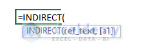
- Syntax:
=INDIRECT(ref_text, [a1])
- Arguments Explanation:
| Argument | Compulsory/Optional | Explanation |
|---|---|---|
| ref_text | Compulsory | Reference of a cell with A1 or R1C1 format. |
| [a1] | Optional | Format of the cell to select- A1 or R1C1 |
- Return Parameter:
The function returns the value(s) present in the stored reference.
Example 1 – Using the INDIRECT Function to Convert a Text String into Cell Reference
- To find the value of B5, enter the formula in B8:
=INDIRECT("B5")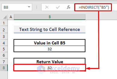
Example 2 – Using the Ampersand to Define the Row and Column Index with the INDIRECT Function
- To find the value of C8, enter the formula in E7:
=INDIRECT("C"&8)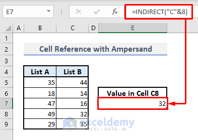
Example 3 – Using the ROW Function inside the INDIRECT Function to Define a Cell Reference
- Enter the formula in F7:
=INDIRECT("C"&ROW())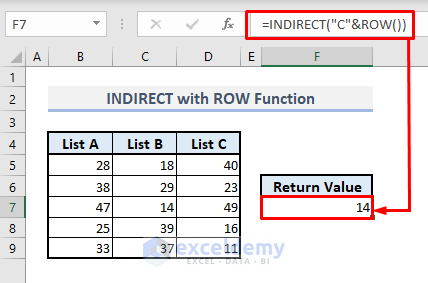
Example 4 – Calculations with Cell References Defined by the INDIRECT Function
- Enter the formula in D9:
=SUM(INDIRECT("B5:B15"))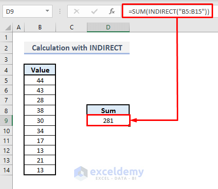
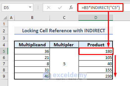
Method 5 – Locking Cell References with the INDIRECT Function in Excel
- To see the output in D5, enter the formula to lock a cell reference in C5:
=B5*INDIRECT("C5")- Press Enter and drag down the Fill Handle to autofill the rest of the cells.
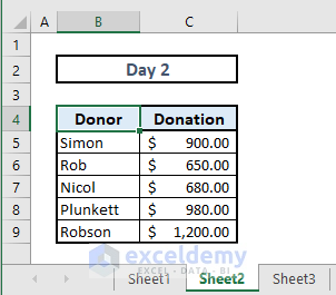
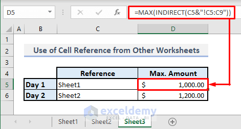
Example 6 – Using a Cell Reference from Another Worksheet with the INDIRECT Function
A chart containing the names of donors and the donation amounts on day 1 is present in Sheet 1.
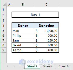
Sheet 2 represents the chart for day 2.
- Enter the formula in D5.
=MAX(INDIRECT(C5&"!C5:C9"))- Press Enter.
You’ll get the value for the first day. Apply the formula to the next output cell to see the maximum amount on the second day.
Read More: How to Use the INDIRECT Function to Get Values from Different Sheet in Excel
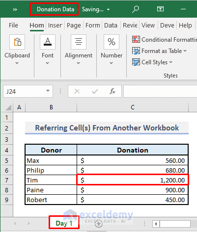
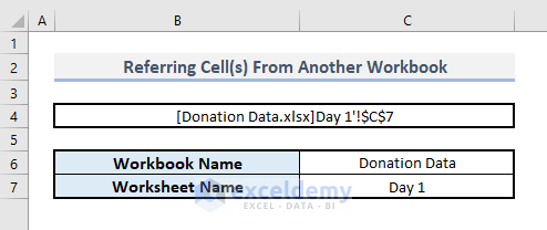
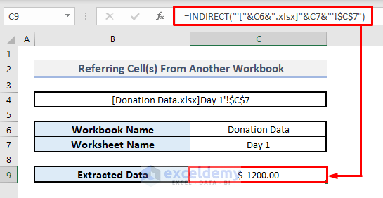
Example 7 – Using a Cell Reference from Another Workbook with the INDIRECT Function
To extract the value of C7 to another workbook:
Step 1:
- Open a new workbook.
- In B4, enter ‘=’ and click C7 in the Donation Data workbook.
Step 2:
- Press Enter. ($1200 is displayed)
- To keep B4 in text format, remove the Equal(=) symbol.
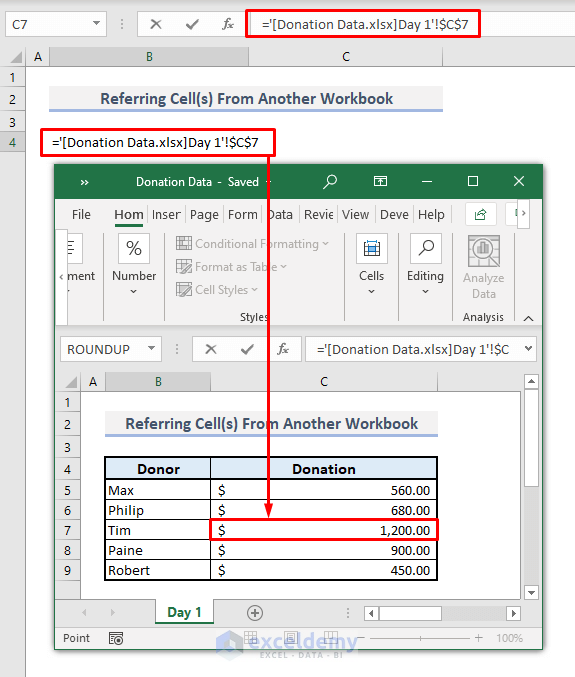
In C6 and C7, enter the names of the Excel workbook and the spreadsheet from which data will be extracted.
Step 3:
- In C9, use:
=INDIRECT("'["&C6&".xlsx]"&C7&"'!$C$7")- Press Enter to see the extracted data.
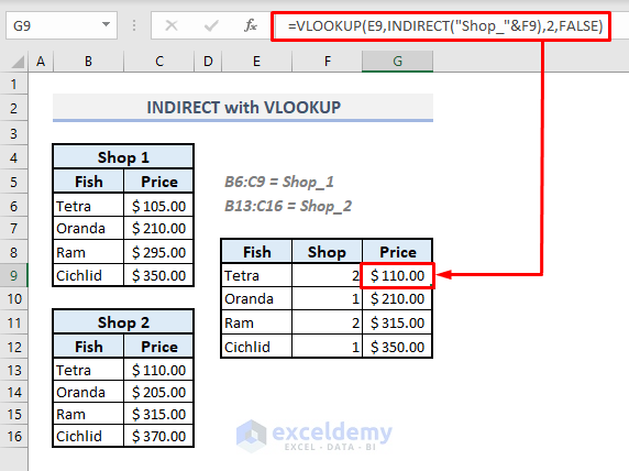
Example 8 – Using the INDIRECT Function to Refer an Array in the VLOOKUP Function
Extract prices to another chart based on the shops.
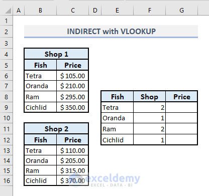
Define fish names and prices in the two different shops. Here, B6:C9 as Shop_1 and B13:C16 as Shop_2.
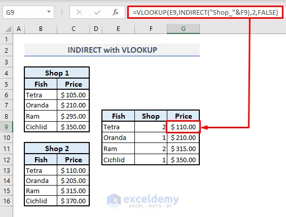
- In G9, extract the price of Tetra in shop 2 using the VLOOKUP function.
The syntax of the VLOOKUP function is:
=VLOOKUP(lookup_value, table_array, col_index_number, [range_lookup])
- Enter the formula in G9:
=VLOOKUP(E9,INDIRECT("Shop_"&F9),2,FALSE)- Press Enter and auto-fill the rest of the cells.
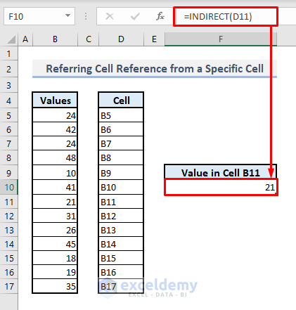
Example 9 – Using the INDIRECT Function to Refer Another Cell Reference from a Specific Cell
- To display the number of B11 in the output cell F10, enter the following formula:
=INDIRECT(D11)- Press Enter to see the result.
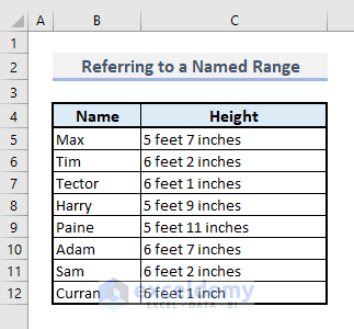
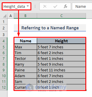
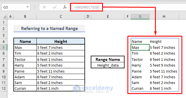
Example 10 – Referring to a Named Range with the INDIRECT Function in Excel
Define the name of this entire table.
Step 1:
- Select the entire table.
- In the Name Box, enter the name of the table: Height_data.
Step 2:
- In E8, define the name of the table.
- Select a random blank cell. Here, G4 and enter:
=INDIRECT(E8)- Press Enter and the entire table will be displayed.
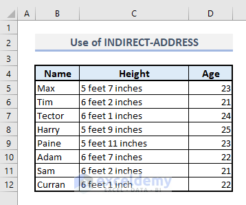
Example 11 – Transposing a Table with the INDIRECT and the ADDRESS Functions in Excel
The syntax of this function is:
=ADDRESS(row_num, column_num, [abs_num], [a1], [sheet_text])
The dataset below showcases name, height, and age.
To transpose the entire table:
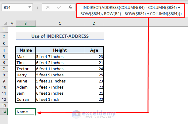
Step 1:
- Select the output cell B14 and enter:
=INDIRECT(ADDRESS(COLUMN(B4) - COLUMN($B$4) + ROW($B$4), ROW(B4) - ROW($B$4) + COLUMN($B$4)))- Press Enter and the formula will return ‘Name’.
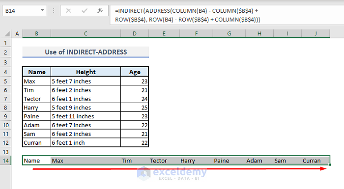
Step 2:
- Drag the Fill Handle to the right.
Step 3:
- Drag down the Fill Handle.
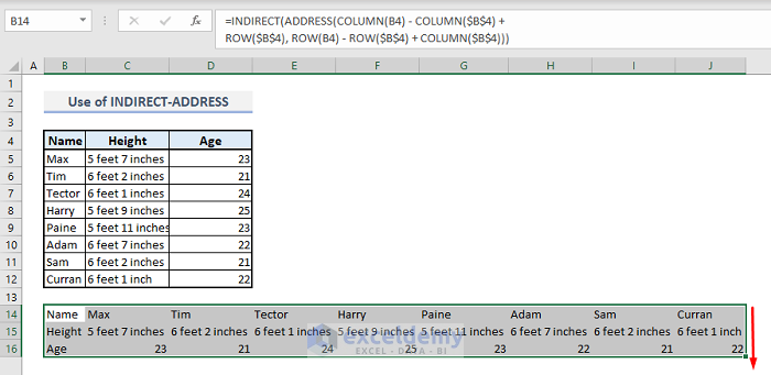
This is the output.
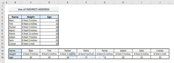
The first argument of the ADDRESS function, “COLUMN(B4) – COLUMN($B$4) + ROW($B$4)” defines the row number by converting the column number of B4.
The second argument, “ROW(B4) – ROW($B$4) + COLUMN($B$4)” defines the column number by converting the row number of B4.
Read More: How to Use INDIRECT ADDRESS Functions in Excel
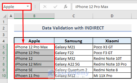
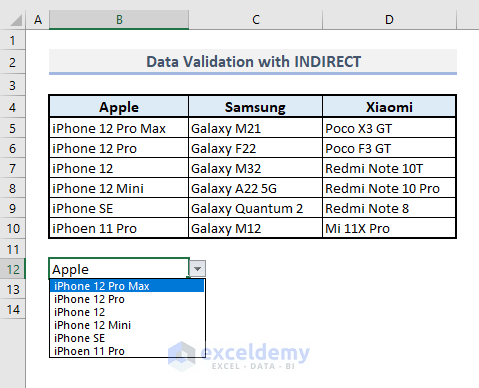
Example 12 – Using the INDIRECT Function for Data Validation in Excel
The dataset showcases 3 smartphone brands, and model names. To create drop-down lists for all smartphone brands:
Step 1:
- Select B5:B10 (model names of Apple products).
- In the Name Box, define the name of this range of cell: Apple.
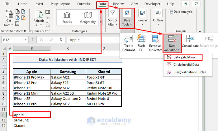
Step 2:
- In B12, enter Apple.
- Select B12.
- Go to the Data tab and choose Data Validation in Data Tools.
Step 3:
- In Allow, choose List.
- In Source, enter:
=INDIRECT(B12)- Press Enter to see the result.
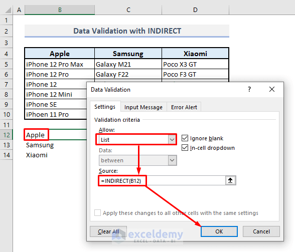
- Go to Cell B12 and you’ll find the drop-down for all Apple products. Follow the same procedure to create drop-downs for the other brands.
The INDIRECT Function Is Not Working in Excel
1. #REF! Error
#REF! Error may be displayed in 3 cases:
- Invalid Cell Reference as ref_text: check the arguments of the function to make sure cell reference valid.
- Exceeding Range Limit: Excel 2007, 2010, and 2013 have a row limit of 1,048,576 and a column limit of 16,384. If you exceed this limit, #REF! Error may occur.
- Using Closed Worksheets or Workbooks: Open the worksheets or workbooks before using them in the function.
2. #NAME? Error
This error occurs for misspelled functions.
Things to Keep in Mind
If you don’t use double-quotes(“ “) while referring to a cell or a range of cells as a text string, the function will return a #REF error.
Unless you define the format of the cell reference in the 2nd argument, the default format will be A1 style.
Download Practice Workbook
Download the Excel workbook.
Excel INDIRECT Function: Knowledge Hub
- Create Drop-Down List Using INDIRECT Function in Excel
- INDIRECT Function with Sheet Name in Excel
- How to Use Excel INDIRECT Range
- How to Convert Text to Formula Using the INDIRECT Function in Excel
<< Go Back to Excel Functions | Learn Excel
Get FREE Advanced Excel Exercises with Solutions!
