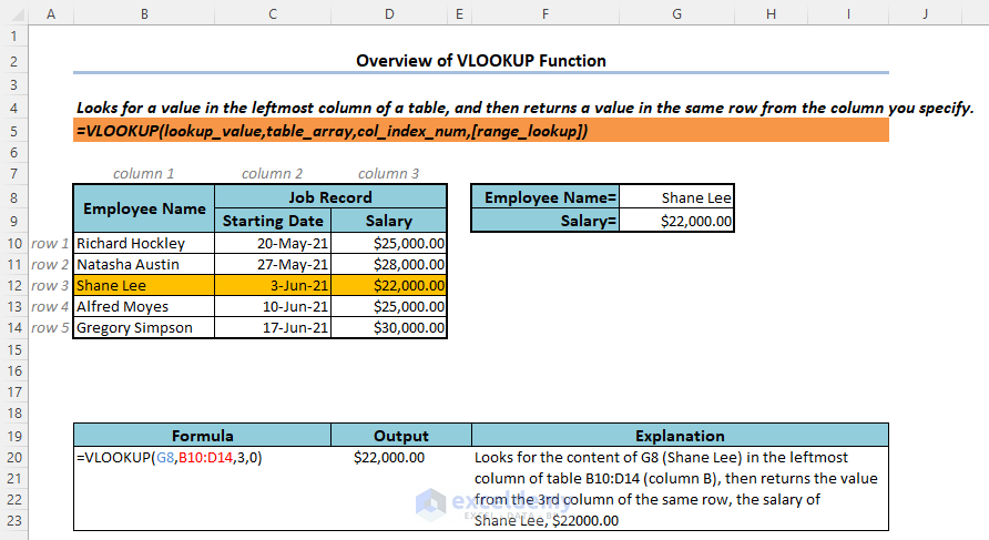
VLOOKUP Function of Excel (Quick View)
The following image is a quick view of Excel VLOOKUP:
Introduction to Excel VLOOKUP Function (Syntax & Argument)
Summary:
The VLOOKUP function looks for a given value in the leftmost column of a given table and then returns a value in the same row from a specified column.
It is available in Excel 2003 and all newer versions.
Syntax:

The Syntax of the VLOOKUP function is:
=VLOOKUP(lookup_value,table_array,col_index_num,[range_lookup])
Arguments:
| Argument | Required/Optional | Value |
|---|---|---|
| lookup_value | Required | The value that it looks for is in the leftmost column of the given table. Can be a single value or an array of values. |
| table_array | Required | The table in which it looks for the lookup_value in the leftmost column. |
| col_index_num | Required | The number of the column in the table from which a value is to be returned. |
| [range_lookup] | Optional | Tells whether an exact or partial match of the lookup_value is required. 0 for an exact match, 1 for a partial match. The default is 1 (partial match). |
Note:
- The lookup_value can be a single value or an array of values. If you enter an array of values, the function will look for each of the values in the leftmost column and return the same row’s values from the specified column.
- The function will look for an approximate match if the [range_lookup] argument is set to 1. In that case, it will always look for the lower nearest value of the lookup_value, not the upper nearest one.
- If the col_index_number is a fraction in place of an integer, Excel itself will convert it into the lower integer. But it will raise #VALUE! error if the col_index_number is zero or negative.
Return Value:
Returns the value of the same row from the specified column of the given table, where the value in the leftmost column matches the lookup_value.
Available in:
Excel 365 | Excel 2021 | Excel 2021 for Mac | Excel 2019 | Excel 2019 for Mac | Excel 2016 | Excel 2016 for Mac | Excel 2013, 2010, 2007 | Excel for Mac 2011 | Excel Starter 2010
How to Use the VLOOKUP Function in Excel: 8 Suitable Examples
When the lookup_value is a single value, it searches for the value in the leftmost column of the given table_array.
- If it finds one, it moves to the specified number of columns right given as col_index_num in the same row.
- The function returns the value from the destination cell.
In the following figure, the formula is:
=VLOOKUP("shane Lee",B6:D10,3,FALSE)
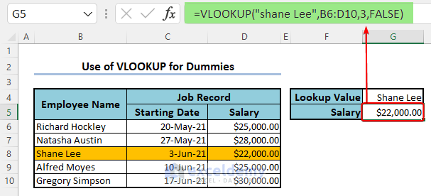
- It searches for “Shane Lee” in the leftmost column B of the table_array B6:D10.
- It finds a result in cell B8. Thus, it moves to column 3 (col_index_num) of the table in the same row, which is cell D8.
- The formula returns the value from that cell. In this case, it is the salary of Shane Lee, $22,000.00.
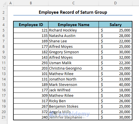
Example 1 – Finding Out the Holder of Maximum Value from a Dataset
Here we have the employee IDs, employee names, and salaries of a company named Saturn Group in columns B, C, and D respectively. We will find out the holder of the maximum ID using the VLOOKUP function.
- Select a destination cell outside the main table.
- The formula will be:
=VLOOKUP(MAX(B5:B21),B5:D21,2,0)
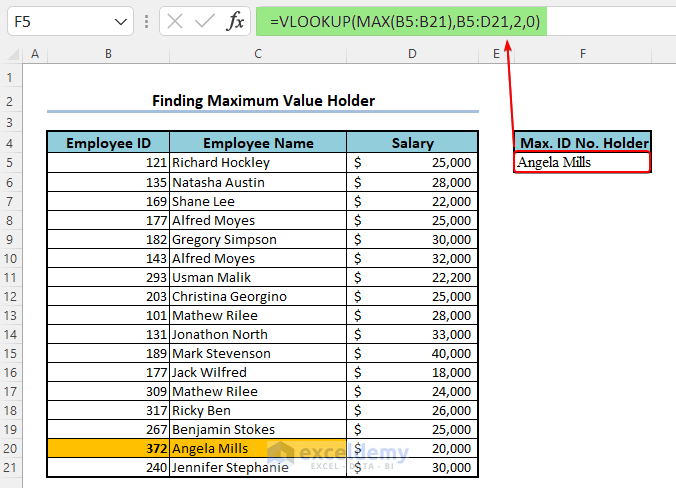
- We have found the Employee with the highest ID, Angela Mills with an ID of 372.
Explanation of the Formula:
- MAX(B5:B21) returns the maximum value between B4 to B20 (Employee IDs). In this case, it is 372. So the formula becomes: VLOOKUP(372,B5:D21,2,0)
- Then it searches for an exact match of the lookup_value 372 in the leftmost column B of the table_array B5:D21. It finds one in cell B20.
- Finally, it moves to column 2 (col_index_num) of the same row, to cell C20. And returns what it gets there. Here it is Angela Mills, the employee with the maximum ID.
Example 2 – Finding Out the Holders of Top n Values from a Dataset
Let’s determine the holders of any top N values from a data set using the VLOOKUP function, for example the employees with the top 5 IDs from the same data set.
- The formula will be:
=VLOOKUP(LARGE(B5:B21,ROW($A$1:$A$5)),B5:D21,2,0)
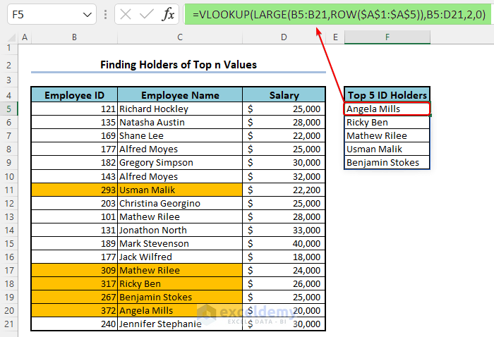
Explanation of the Formula:
- ROW(A1:A5) returns an array of numbers from 1 to 5, {1,2,3,4,5}. For details, see this article.
- LARGE(B5:B21,ROW(A1:A5)) becomes LARGE(B5:B21,{1,2,3,4,5}). It then returns the top 5 IDs from cells B5 to B21. These are: {372,317,309,293,267}.
- VLOOKUP(LARGE(B5:B21,ROW(A1:A5)),B5:D21,2,0) then becomes VLOOKUP({372,317,309,293,267},B5:D21,2,0). It is a combination of a total of 5 formulas.
♦ VLOOKUP(372,B5:D21,2,0)
♦ VLOOKUP(317,B5:D21,2,0)
♦ VLOOKUP(309,B5:D21,2,0)
♦ VLOOKUP(293,B5:D21,2,0)
♦ VLOOKUP(267,B5:D21,2,0)
- VLOOKUP(372,B5:D21,2,0) searches for an exact match of 372 in the leftmost column B of table B5:D21. After finding one, it moves to the 2nd column of the same row of the table, then returns the name of the employee. In this case, Angela Mills.
- The formula then repeats the check for other values. Thus we get the list of the employees with the top 5 salaries.
Note:
This is an array formula, so press Ctrl + Shift + Enter to apply it unless you are in Office 365.
Read More: 7 Practical Examples of VLOOKUP Function in Excel
Example 3 – Find an Approximate Match with Excel VLOOKUP Function
In the case of an approximate match (when the [range_lookup] argument is zero), the function always looks for the lowest nearest match.
- In the following example, the formula is:
=VLOOKUP(G4,B5:D9,2,1)

- The [range_lookup] argument is 1, so it searches for an approximate match.
- The lookup_value is 168. It settles in 135, the lower nearest value to 168, and returns the corresponding Employee Name, Natalia Austin.
- While the upper nearest value 169 is far closer, the formula ignores closeness.
Read More: How to Use VLOOKUP Function with Exact Match in Excel
Example 4 – Match Multiple Lookup Values with Excel VLOOKUP Array Formula
When the lookup_value is an array of values in place of a single value, the function searches for each of the lookup_values in the leftmost column of the table_array one by one.
- In the following figure, the formula is:
=VLOOKUP(G4:H4,B6:D10,3,FALSE)
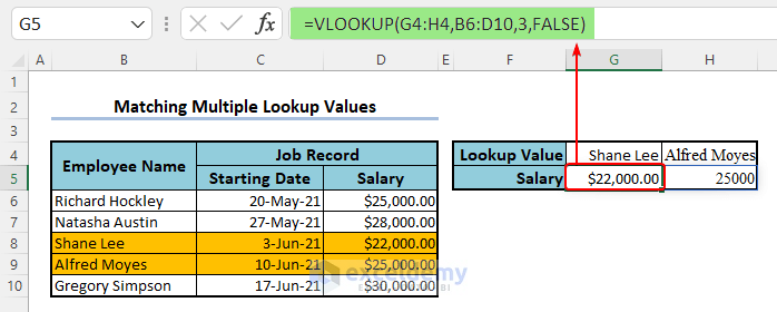
- It searches for G4 (Shane Lee) in the table and returns his salary, $22000.
- Then, it searches for H4 (Alfred Moyes) in the table and returns his salary, $22000.
Note:
Note that you have to press Ctrl + Shift + Enter to enter an array Formula unless you are in Office 365.
Example 5 – Combine the CHOOSE Function with Excel VLOOKUP to Match Multiple Conditions
The VLOOKUP function can be used to extract data for multiple criteria lookups when combined with CHOOSE, IF, or MATCH functions. Here we have the Brand, Model, Chipset, RAM, and Price data of some mobile phone companies.
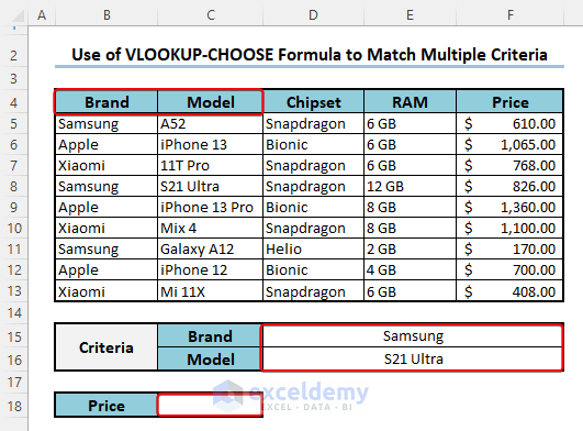
- We set two criteria, Brand and Model, to get the corresponding Price in cell C18.
- The formula will be:
=VLOOKUP($D$15&$D$16,CHOOSE({1,2},$B$5:$B$13&$C$5:$C$13,$F$5:$F$13),2,FALSE)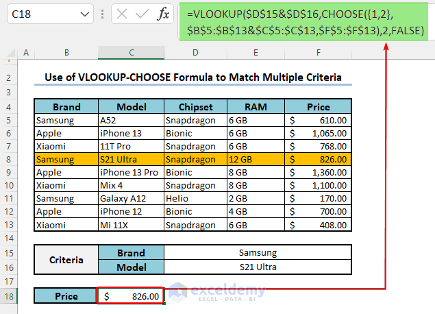
Read More: 10 Best Practices with VLOOKUP in Excel
Example 6 – Use a Helper Column and Merge VLOOKUP with the MATCH Function for Multiple Criteria
Let’s use the same dataset from the previous example.
- Create a helper column to concatenate the Brand and Model columns with the following formula:
=C5&D5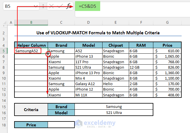
- Apply the following formula in the output cell to get the desired result:
=VLOOKUP(D15&D16,B5:G13,MATCH(B18,B4:G4,0),FALSE)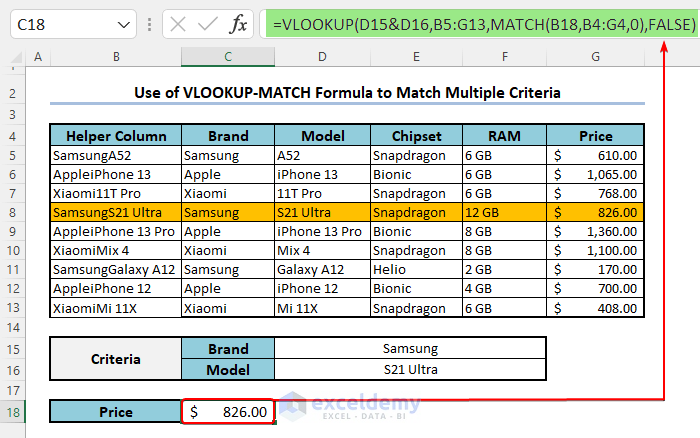
Read More: INDEX MATCH vs VLOOKUP Function
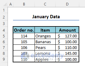
Example 7 – Combine VLOOKUP with INDIRECT Function to Lookup Across Spreadsheets
We have 4 sheets named Jan, Feb, Mar, and Apr with the data for the months of January, February, March, and April. Here’s how one of them looks.
- Create another sheet that contains the datasheet names. You have to write the names of the sheets accurately to avoid errors.
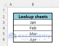
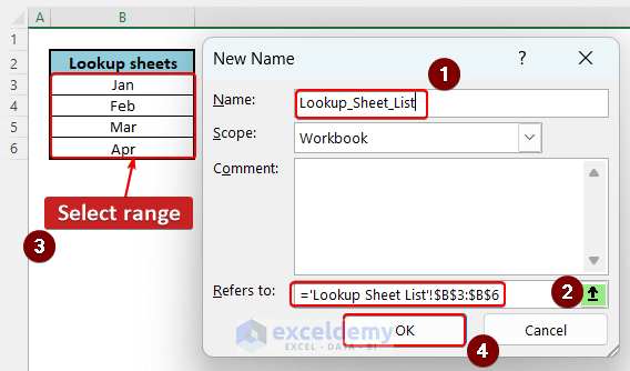
- Create a named range for the new range B3:B6.
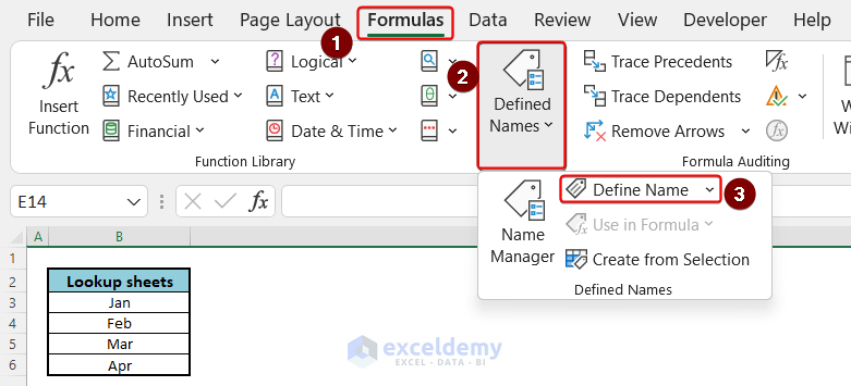
- Create the named range and name it Lookup_Sheet_List.
- If your name contains multiple words, you have to put underscores in between.
- Go to your main sheet where you want to perform lookup operations. Here, we are looking up Order nos.
- In cell C5, copy the following formula:
=IFNA(VLOOKUP($B5, INDIRECT("'"&INDEX(Lookup_Sheet_List,MATCH(1, --(COUNTIF(INDIRECT("'" & Lookup_Sheet_List &"'!$B$3:$B$6"), $B5)>0), 0)) & "'!$B$5:$D$9"), 2, FALSE), "Not found")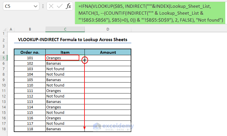
- To get Amounts, copy the following formula in the column next to it.
=IFNA(VLOOKUP($B5, INDIRECT("'"&INDEX(Lookup_Sheet_List,MATCH(1, --(COUNTIF(INDIRECT("'" & Lookup_Sheet_List &"'!$B$3:$B$6"), $B5)>0), 0)) & "'!$B$5:$D$9"), 3, FALSE), "Not found")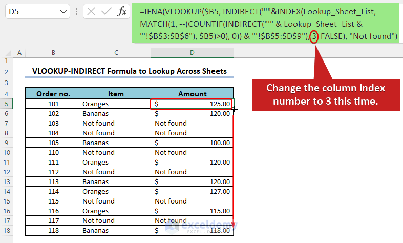
- You have to change the column index number accordingly.
Example 8 – Using the VLOOKUP Function to Lookup to the Left
This time, we want to look up the Employee’s Name and get the corresponding ID.
- The formula will be:
=VLOOKUP(G4,IF({1,0},C5:C9,B5:B9),2,0)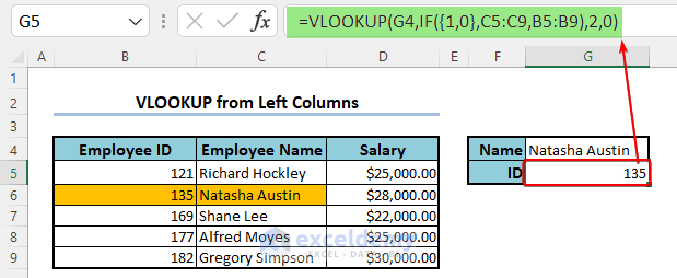
Here, {1,0} inside the IF function is important. If you alter the sequence, i.e. put {0,1} instead, the formula will not work as expected.
Read More: Excel LOOKUP vs VLOOKUP: With 3 Examples
Common Errors with Excel VLOOKUP Function
The VLOOKUP function has the following common errors.
| Error | When They Show |
|---|---|
| #N/A! | Shows when it does not find a match of the lookup_value in the leftmost column. |
| #VALUE! | Show when an argument of the function is of the wrong data type. For example, when the col_index_number is negative, or a text or the [range_lookup] argument is not 0 or 1. |
Limitations of Excel VLOOKUP Function
Though VLOOKUP is one of the most used functions in Excel, it has some limitations:
- You can’t use it when the lookup_value is in a column right next to the required value.
For example, in example 1, you can not use the VLOOKUP function if you are asked to find out the employee with the maximum salary because the salary is in a column right to the required value, the employee name.
You can use the XLOOKUP or INDEX-MATCH functions of Excel to come out of this limitation.
- If you have the same lookup_value more than once in the table, the VLOOKUP function will only provide you with information about the first one it gets.
For example, in the data set of example 1, there are two employees named Mathew Rilee. Now if we want to get the salary of Mathew Rilee, we will only get the salary of the first one, $28000.

You can solve this problem using the FILTER function.
- In the case of an approximate match, the VLOOKUP function always settles for the lower nearest value of the lookup_value, even when the upper nearest value is closer.
- The VLOOKUP function does not update automatically when you insert a new column. To get rid of this problem, you can use the INDEX-MATCH function of Excel.
Download Practice Workbook
You can download the following practice workbook that we used to write this article.
Excel VLOOKUP Function: Knowledge Hub
<< Go Back to Excel Functions | Learn Excel
Get FREE Advanced Excel Exercises with Solutions!

Thanks for your teaching in Excel. You gave me a lot of insight into the new features of Excel 365
Hello, Ruben!
It’s glad to know that our content is helpful to you. To know more about Excel stay in touch with ExcelDemy.
Regards
ExcelDemy