Brief Description of the VLOOKUP Function
In the below example, there is a movie dataset. Here, we used the VLOOKUP formula to extract data.
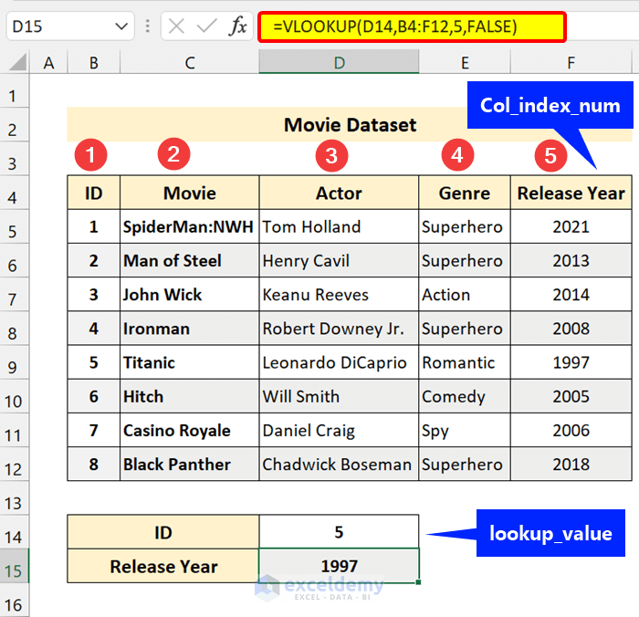
In this VLOOKUP formula:
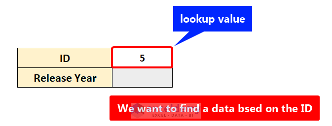
Our lookup_value is 5, which is ID.
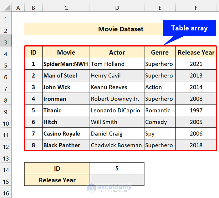
Our table array is B4:F12
Range lookup is set to FALSE for the Exact match.
The column index number is 5, which is the Release Year.
We are telling the VLOOKUP function to search the table array with an ID 5. If you found that, then give the value presented in the column Release Year, which has a column index number of 5.
6 Things You Should Know About ‘Column Index Number’ of VLOOKUP
1. What Does Column Index Number Do?
Why is the column index number essential, and what does it do in the formula? Let’s break it down from the previous example.
The formula we are using:
=VLOOKUP(D14,B4:F12,5,FALSE)
We set the range lookup to FALSE for the exact match.
Breakdown 1: Lookup a Value
To find the value, we must provide a lookup value in the VLOOKUP formula. First, we have to give the lookup value for which it will search the data. We are using cell references here.
Breakdown 2: Initialize the Table Array
The VLOOKUP function will look for the Table Array.
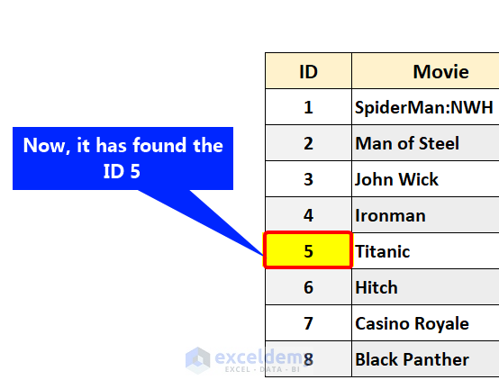
Breakdown 3: Look for the Lookup value in the leftmost column
VLOOKUP will search the lookup value vertically from the leftmost column of the table array.
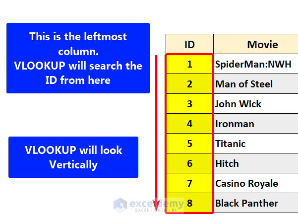
As we set the range lookup argument to FALSE to find an exact match, it will find one.
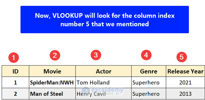
Breakdown 4: Look for the Column Index Number from Table Array
The VLOOKUP function will try to find the column number from the table entered in the argument.
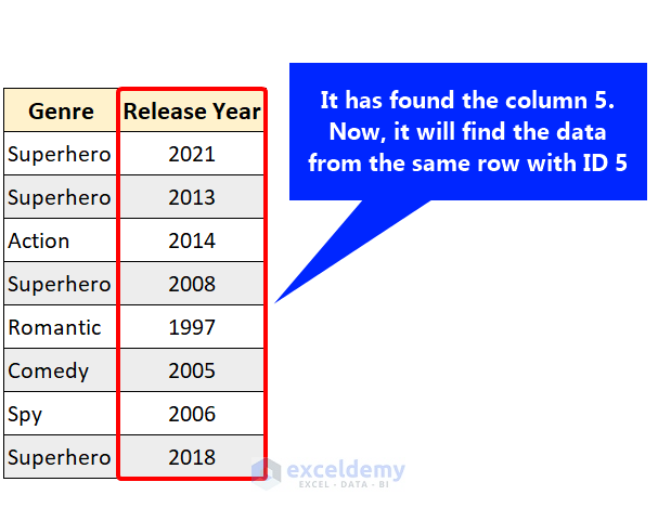
Breakdown 5: VLOOKUP Looks for Value in the Given Column Index Number
After it has found the desired column, VLOOKUP will search for your value in the column that shares the same row with ID 5.
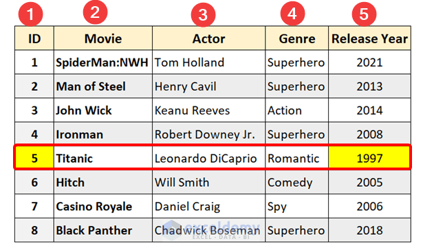
Breakdown 6: Return the Value
It will find the Release Year with the ID 5.
2. How Do Outputs Vary Based on Column Index Number?
Our VLOOKUP formula will return a different result based on the different column index numbers.
When you want an alternate result from the table, make sure you provide the correct column index number in the function. Your outputs will vary based on this column range.
Take a look at the following example:
The formula:
=VLOOKUP(D14,B4:F12,3,FALSE)
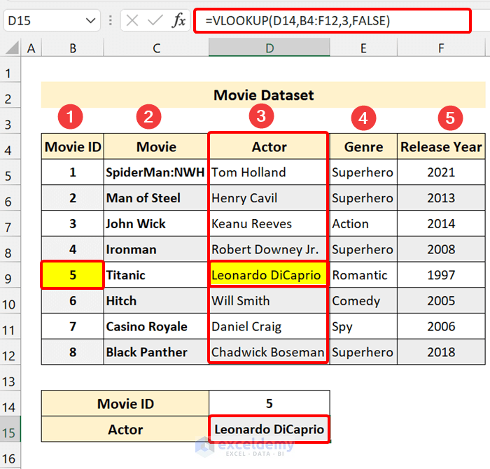
We wanted the Actor’s name from Movie ID 5. Our actor column is the third column in the table array. We provided 3 as a column index number in the VLOOKUP formula. Our function fetched the value from range to lookup (the table array) in Excel.
3. What Happens If We Give a Wrong Column Index Number?
If your desired result column doesn’t match the column index number you have given, you won’t get the result.
Take a look at the following example:
The formula:
=VLOOKUP(D14,B4:F12,5,FALSE)
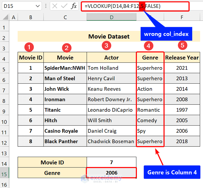
Here, you can see we wanted the Genre of Movie ID 7. But it shows 2006, which is an incorrect answer.
We provided 5 as a column index number in the Excel VLOOKUP formula, but the column number of Genre is 4. That’s why it is returning a different result.
4. What Happens If Our Column Index Is Out of Range?
If your column index number is out of range from the given table array, the VLOOKUP function will return the #REF! error. It is because your table array doesn’t contain that many columns.
You can understand this from the following example:
The formula:
=VLOOKUP(D14,B4:F12,6,FALSE)
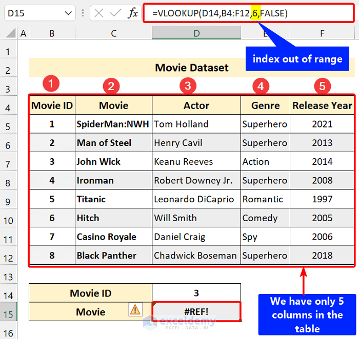
Our Excel VLOOKUP formula is showing an error. Our table array is B4:F12. In this range, we have only five columns, but in our formula, we provided 6 in the col index argument.
5. Column Index Number Increase in VLOOKUP Using COLUMN Function
You can use the dynamic column index in the VLOOKUP formula. Suppose you have two tables and want to merge them. You also need to copy a working VLOOKUP formula in multiple columns. A handy way to do this is to use the COLUMN function of Excel.
Take a look at the following screenshot:
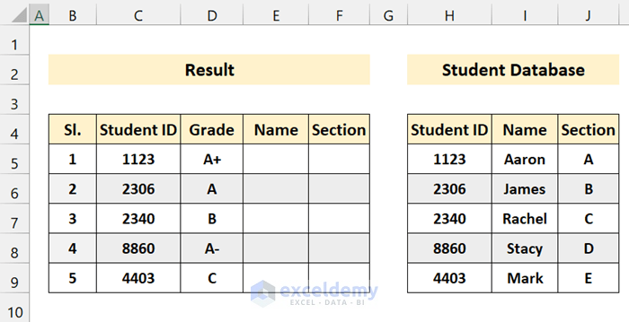
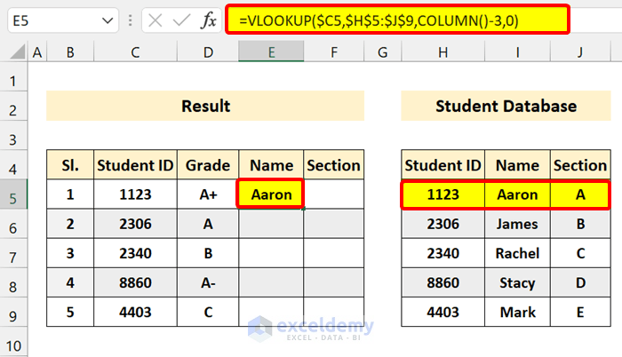
We have two tables here. Based on student ID, we want to merge the Result table and the Student Database table. Our goal is to set the Name and section in the Result table.
The formula:
=VLOOKUP($A1,table,COLUMN()-x,0)
- Enter the following formula in Cell E5 and press Enter:
=VLOOKUP($C5,$H$5:$J$9,COLUMN()-3,0)
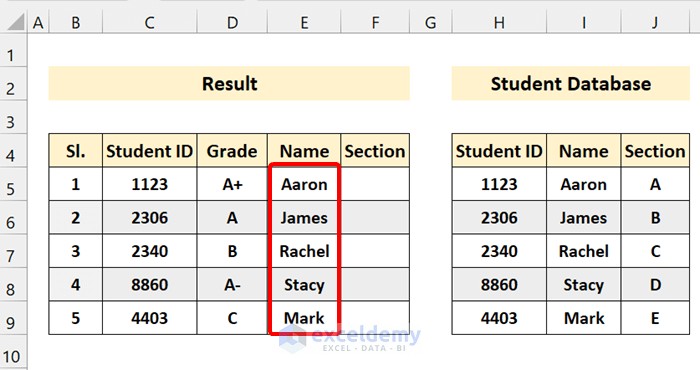
- Drag the Fill handle icon across the table.
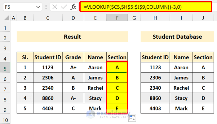
- Enter the formula in Cell F5 and drag the Fill handle icon:
Note: You can use this formula as a Column Index Number Calculator for VlOOKUP in your worksheet.
Breakdown of the Formula
We calculated the column index number utilizing the COLUMN function. If the COLUMN function does not take arguments, it returns the number of the related column.
Now, as we are using the formula in Columns E and F, the COLUMN function will return 5 and 6, respectively. In the sheet, column E’s index number is 5, and Column F‘s index number is 6.
We don’t like to get data from the 5th column of the Result table (there are only 3 columns total). Subtract 3 from 5 to acquire the number 2, which the VLOOKUP function used to recover Name from the Student Database table.
COLUMN()-3 = 5-3 = 2 (Here, 2 indicates the Name column of the Student Database table array)
We used the same formula in Column F. Column F has index number 6.
COLUMN()-3 = 6-3 = 3 (3 indicates the Section of Student Database table array)
The first sample uses the Name from the Student Database table (column 2), and the second illustration uses the Section from the Student Database table (column 3).
[/wpsm_box]6. Find Column Index Number with MATCH Function
Here, we have a dataset with students’ grades in Physics, Math, and Chemistry. We want to find the Grade of Jessy in the Math subject.
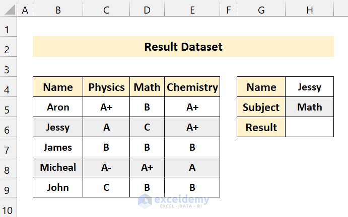
- Enter the following formula in Cell H5 and press Enter:
=VLOOKUP(H4,B4:E9,MATCH(H5,B4:E4,0),FALSE)
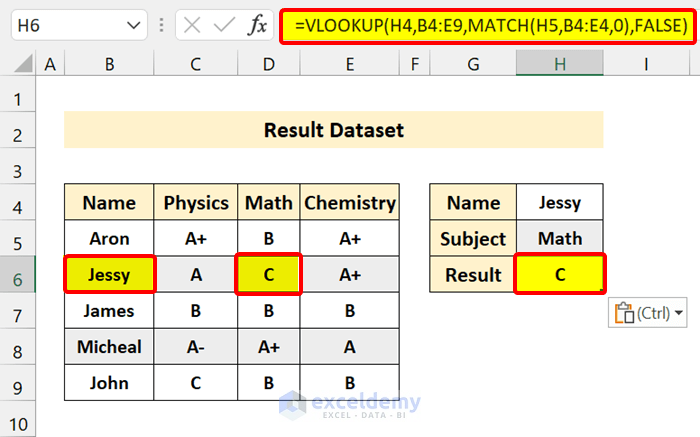
The VLOOKUP formula has gained the exact match from the dataset.
We didn’t provide a static number in the column index number. Instead, we made it dynamic by using the MATCH function. We have a multiple set of criteria.
Breakdown of the Formula
➤ MATCH(H5,B4:E4,0)
The MATCH function will search for the subject MATH from the header B4:E4. It will find it in index 3. That’s why it will return 3.
➤ VLOOKUP(H4,B4:E9,MATCH(H5,B4:E4,0),FALSE) = VLOOKUP(H4,B4:E9,3, FALSE)
It will work like the actual VLOOKUP formula. And it will return C. Because the value was found in column index number 3.
VLOOKUP Column Index Number from Another Sheet or Workbook
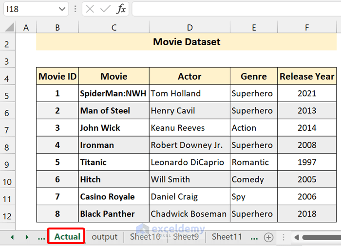
Here, we have two separate sheets. Our main dataset is in the Actual sheet. We will get the data from here and enter it into the output sheet. We are using a column index number where our table array is located on another sheet.
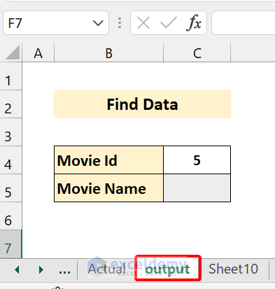
Enter the following formula in Cell C5 of the output sheet and then press Enter.
=VLOOKUP(C4,Actual!B4:F12,2,FALSE)
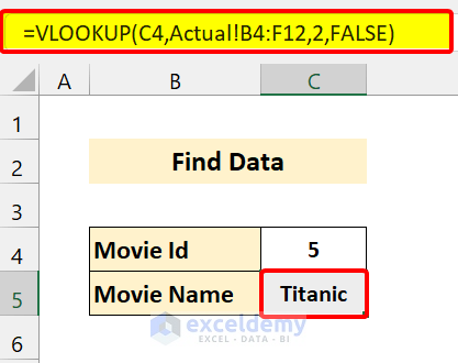
The VLOOKUP column index number helped us get data from another sheet.
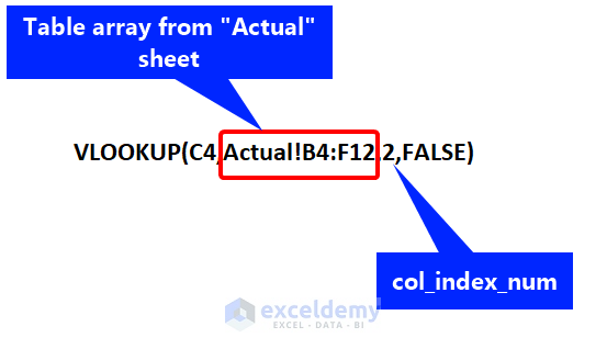
The formula “Actual!B4:F12” indicates the sheet name and the table array from the sheet. We gave 2 as a column index number to get data from the table in the “Actual” sheet.
The same goes for the various workbooks. You can similarly fetch a value from another workbook using the VLOOKUP function. T
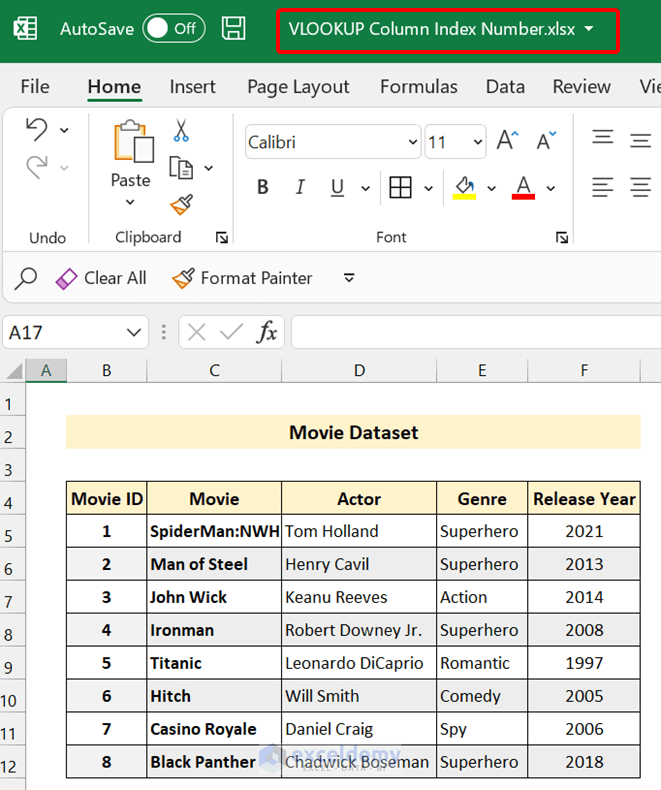
This is the first workbook. We have our data – “Actual” sheet:
This is the second workbook. We will show the value in the “Data” sheet.
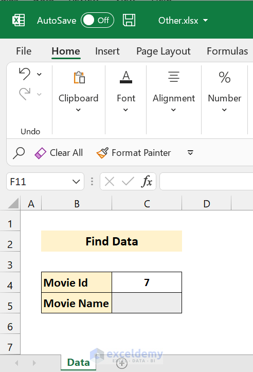
Enter the following formula in Cell C5 of the “Data” sheet from the “Other.xlsx” workbook:
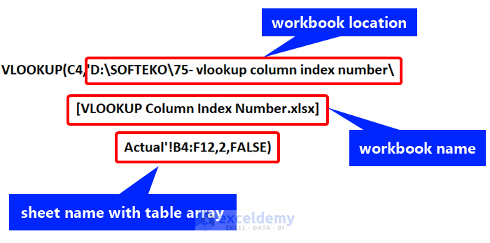
=VLOOKUP(C4,'[VLOOKUP Column Index Number.xlsx]Actual'!B4:F12,2,FALSE)
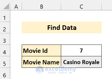
It returned an exact match from the dataset.
If you close the main workbook where your table array is, the formula will look like the following:
=VLOOKUP(C4,'D:\SOFTEKO\75- vlookup column index number\[VLOOKUP Column Index Number.xlsx]Actual'!B4:F12,2,FALSE)
Things to Remember
✎ VLOOKUP searches value in the right direction.
✎ To get accurate results, provide a valid column index number. The column index number should not exceed the table array column number.
✎ You should lock the table array range if you are conveying the data from the same worksheet or other worksheets but the exact workbook.
Download the Practice Workbook
Download the following practice workbook.
Related Articles
- How to Use VLOOKUP for Multiple Columns in Excel
- VLOOKUP from Multiple Columns with Only One Return in Excel
- How to Use VLOOKUP to Return Multiple Columns in Excel
- How to Use VLOOKUP Function to Compare Two Lists in Excel
- How to Use the VLOOKUP Ascending Order in Excel
- VLOOKUP with Drop Down List in Excel
- How to Use VLOOKUP for Rows in Excel
- Perform VLOOKUP by Using Column Index Number from Another Sheet
- How to Find Column Index Number in Excel VLOOKUP
<< Go Back to Excel VLOOKUP Function | Excel Functions | Learn Excel
Get FREE Advanced Excel Exercises with Solutions!

This is useful. Thanks a lot.
I don’t understand why though, in the first 4 paragraphs, columns are indexed as such: column B’s index is 1, column C’s index is 2,…, column E’s index is 4 and column F’s index is 5″…
… But on the 5th paragraph “5. VLOOKUP Column Index Number Increase Using the COLUMN Function”, it is said that column E’s index is 5 and column F’s index is 6: “*Now, as we are using the formula in Column E and F, the COLUMN function will return 5 and 6 respectively. In the sheet, column E’s index number is 5. And column F’s index number is 6.*”
Hello Thanks,
In the first 4 paragraphs, we use =VLOOKUP(D14,B4:F12,5,FALSE) this formula. Here, we define the range of cells. So, when we define column number as 5, Excel will count from column B as the first column.
Whereas, =VLOOKUP($C5,$H$5:$J$9,COLUMN()-3,0) in this equation, we use Column() function. This function will count the column number from column A. So, when you have COLUMN()-3 and are in column E, it will be 5-3= 2.
So, I hope you understand it clearly. If you have further queries, feel free to ask in the comment box.