Here we have a dataset of equipment lists for two gyms. We will compare the lists using the VLOOKUP function.
Method 1 – Compare Two Lists in the Same Sheet Using the VLOOKUP Function in Excel
We will compare whether the equipment from Gym 2 is present within the Gym 1 equipment list.
Part 1 – Basic Steps
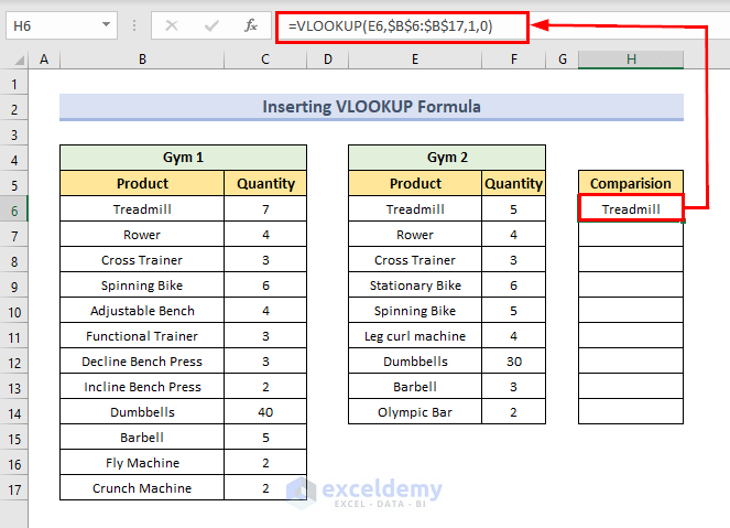
- Insert the following formula in Cell H6.
=VLOOKUP(E6,$B$6:$B$17,1,0)- Press Enter.
In the formula, we have set the element from Gym 2 as lookup_value and the equipment from Gym 1 as lookup_array. This will return the equipment name when it is found within the Gym 1box.
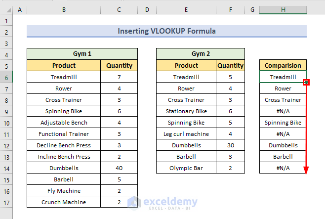
- Use the Fill Handle to copy the formula in the cells below.
- We will see the result in every cell.
Part 2 – Use the ISNA Function for Error Handling
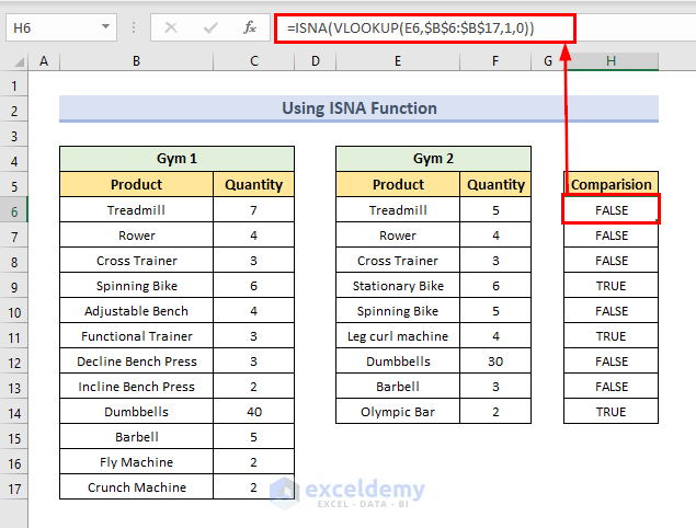
ISNA checks whether a value is #N/A, and returns TRUE or FALSE.
- Use the following formula in Cell H6.
=ISNA(VLOOKUP(E6,$B$6:$B$17,1,0))- Press Enter.
- Use the Fill Handle to copy the formula in the following cells.
- We will see the result in every cell as True or False.
Part 3 – Apply an Additional NOT Function to Clarify Results
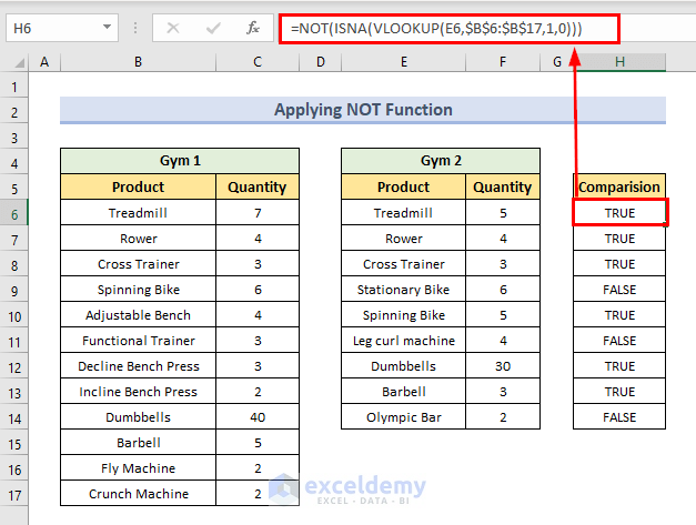
- Use the following formula in Cell H6.
=NOT(ISNA(VLOOKUP(E6,$B$6:$B$17,1,0)))- Press Enter and use the Fill Handle to copy the formula in the following cells.
- This will return TRUE when the item is found within the list and for comparing a value that is not within the list the formula will return FALSE.
Part 4 – Insert the IF Function for Inputting Text Value
- Use the following formula in Cell H6 and press Enter.
=IF(NOT(ISNA(VLOOKUP(E6,$B$6:$B$17,1,0))),"Found","Not Found")- Use the Fill Handle to copy the formula in the following cells.
- This will put Found or Not Found in every cell rather than the Boolean values.
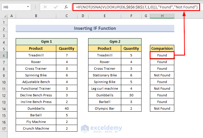
- In the condition check field of IF, we have inserted the previously used NOT-ISNA-VLOOKUP formula.
- We have set “Found” and “Not Found” as the if_true_value and if_false_value respectively.
- When the condition is TRUE (equipment is in the list) the formula will return “Found.”
- And when the condition is FALSE (equipment is not in the list) the formula will return “Not Found.”
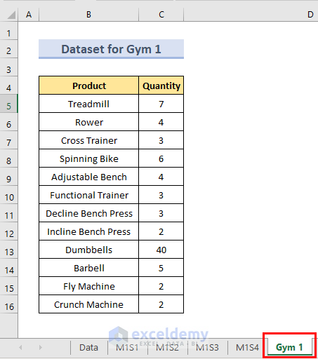
Method 2 – Compare Two Lists in Different Sheets Using the VLOOKUP Function in Excel
Here we have Gym 1 equipment in the Gym 1 sheet, while the items for Gym 2 are in sheet M2.
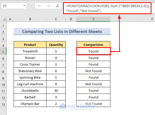
We will compare the values in the second sheet.
Steps:
- Open the sheet where we will do the comparison.
- In Cell E5, use the following formula.
=IF(NOT(ISNA(VLOOKUP(B5,'Gym 1'!$B$5:$B$16,1,0))),"Found","Not Found")- Press Enter and use the Fill Handle to copy the formula in the following cells.
Note:
- We are comparing in the M2 sheet, so we need to provide this sheet name, but the lookup_array value is in the separate sheet Gym 1. That is we need to provide the sheet name so that, Excel can understand where to find it.
- After providing the sheet name make sure to insert an exclamatory sign (!). And if the sheet name has multiple words then put the name within a single quote (”).
Read More: VLOOKUP Example Between Two Sheets in Excel
An Alternative for VLOOKUP for Comparing Two Lists in Excel
Instead of VLOOKUP, we can use the COUNTIF function.
- Use the following formula in Cell H6.
=IF(COUNTIF($B$6:$B$17,E6)<>0,"Found","Not Found")- Press Enter and use the Fill Handle to copy the formula in the following cells.
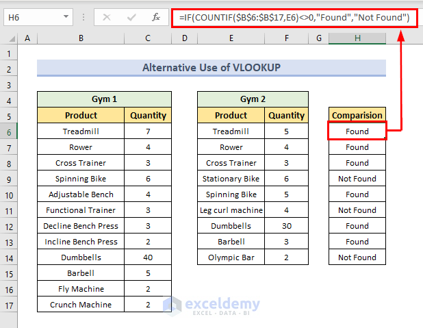
- Within the COUNTIF we have checked whether occurrences of the lookup value are not equal to 0 or not.
- If not 0 (means the product presents in the list), then it returns “Found”, otherwise “Not Found”.
Download the Practice Workbook
Further Readings
- How to Use VLOOKUP for Multiple Columns in Excel
- VLOOKUP from Multiple Columns with Only One Return in Excel
- How to Use VLOOKUP to Return Multiple Columns in Excel
- How to Use the VLOOKUP Ascending Order in Excel
- VLOOKUP with Drop Down List in Excel
- How to Use VLOOKUP for Rows in Excel
- How to Use Column Index Number Effectively in Excel VLOOKUP
- Perform VLOOKUP by Using Column Index Number from Another Sheet
- How to Find Column Index Number in Excel VLOOKUP
<< Go Back to VLOOKUP a Range | Excel VLOOKUP Function | Excel Functions | Learn Excel
Get FREE Advanced Excel Exercises with Solutions!
