Excel VLOOKUP to Find Last Value in Column (with Alternatives)

Finding a value in a column – a vertical lookup – is a common task when working in Excel. Excel provides a built-in VLOOKUP function for this purpose, but this has limitations, To work round these, we can make our own formulas that will work as vertical lookup to return values with more dynamic criteria. In this article, we will examine how to find the last value in a column with VLOOKUP, the limitations of this method, and several alternative methods.

Using the VLOOKUP Function to Find Last Value in Column

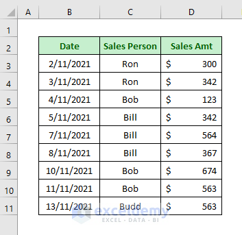
Let’s get introduced to our sample dataset first. It has 3 columns and 10 rows to containing some salespersons’ sales amounts on particular dates.

We’ll find the last occurrence of a value by using the VLOOKUP Function.

Specifically, we have 3 different sales amounts for Bill. Let’s find the amount of his last sales and place it in Cell G5.

Steps:

• In Cell G5, enter the formula below:

• Press Enter to return the last occurrence of his sales.

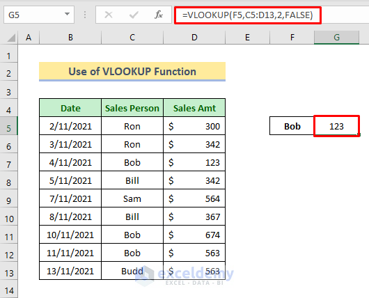
The result is incorrect, because the lookup data is unsorted.

VLOOKUP will return an error for unsorted data in approximate mode.

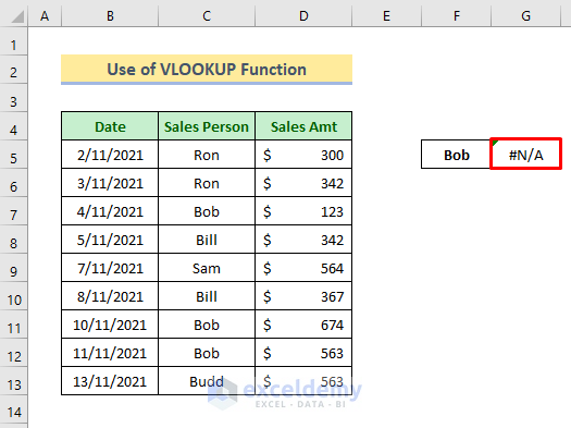
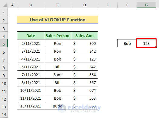
And if, as we did in the formula above, we use exact match for the fourth argument in the formula, the first match will be returned, not the last. That’s because VLOOKUP uses binary search, so when it finds a value larger than the lookup value, it reverts to the previous matched value.

Alternatives to VLOOKUP to Find Last Value in Column

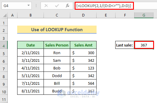
Method 1: Using the LOOKUP Function

The LOOKUP function is used for looking through a single column or row to find a particular value from the same place in a second column or row.

Steps: 

• Activate Cell G4.
• Enter the formula below:

• Press Enter to return the last value.

Formula Breakdown:

• D:D<>””

Checks if the cells in Column D are empty or not. It will return as-

{FALSE;FALSE;FALSE;TRUE;TRUE;TRUE;TRUE;TRUE;TRUE;TRUE;FALSE…..}

• 1/(D:D<>””)

Divides 1 by the result. As FALSE means 0 and TRUE means 1 the result will be as follows:

{#DIV/0!;#DIV/0!;#DIV/0!;1;1;1;1;1;1;1;#DIV/0!;#DIV/0!}

• LOOKUP(2,1/(D:D<>””),D:D)

We set the lookup value to 2 because the lookup function will find 2 through the column. When it reaches an error then it will return to its nearest value of 1 and will show that result. That will return as:

367

Read More: How to Use VLOOKUP to Find Duplicates in Two Columns

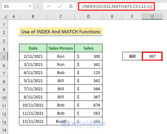
Method 2 – Using INDEX and MATCH Functions

The INDEX function returns a value or the reference to a value from within a table or range. The MATCH function is used to search for a specified item in a range and return the relative position of that item in the range.

Steps:

• Enter the formula below in Cell G5:

• Press Enter.

How Does the Formula Work:

• MATCH(F5,C5:C13,1)

Here the MATCH function is used to find the value of Cell F5 for items sorted in ascending order from the array C5:C13. Setting the third argument to ‘1’  indicates an approximate match. The function will return as-

6

This is the row number counted from the first entry.

• INDEX(D5:D13,MATCH(F5,C5:C13,1))

The INDEX function will give the corresponding sales (D5:D13) according to the previous match from the array (C5:C13), which will return as-

367

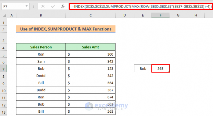
Method 3 – Combining INDEX, MAX, SUMPRODUCT And ROW Functions

The ROW function finds row numbers. SUMPRODUCT is a function that multiplies a range of cells or arrays and returns the sum of the products. The MAX function will find the maximum number. The INDEX function returns a value or the reference to a value from within a table or range.

Steps:

• Enable editing in Cell F7.
• Copy and paste the formula below:

➦ Press Enter.

How Does the Formula Work:

• ROW($B$5:$B$13)

The ROW function will show the row number for the array that will return as-

{5;6;7;8;9;10;11;12;13}

• ($E$7=$B$5:$B$13)

Here Cell E7 is our lookup value and this formula will match it through the array B5:B13. It will return as-

{FALSE;FALSE;FALSE;FALSE;TRUE;FALSE;FALSE;FALSE;TRUE}

• ROW($B$5:$B$13)*($E$7=$B$5:$B$13)

This is the multiplication of the previous two formulas that will actually multiply the corresponding row numbers. FALSE means 0 and TRUE means 1. So after multiplication, it will return as-

{0;0;0;0;9;0;0;0;13}

• MAX(ROW($B$5:$B$13)*($E$7=$B$5:$B$13))

The MAX function will find the maximum value from the previous result, that will return as

13

• SUMPRODUCT(MAX(ROW($B$5:$B$13)*($E$7=$B$5:$B$13))-4)

The SUMPRODUCT function is used to find the row number in the array. As our list starts from the 5th row onwards, 4 has been subtracted. So the position of the last occurrence of Bill is 9 on our list, so the formula will return as-

9.

INDEX($C$5:$C$13,SUMPRODUCT(MAX(ROW($B$5:$B$13)*($E$7=$B$5:$B$13))-4))

The INDEX function is used to find the sales for the last matched name. And it will return as-

563

That is our last occurrence for Bill.

Method 4 – Use Excel VBA to Find Last Occurrence of a Value in Column

We can perform the previous operation by using VBA code.

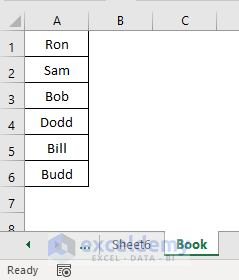
First, we’ll make a dropdown bar for the unique names. Then we’ll make a new user-defined function “LastItemLookup” using VBA and use it to find the last occurrence.

Steps:

• Copy the unique names from the main sheet to a new sheet.

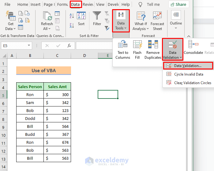
• Go to the main sheet and activate any new cell, here E5.
• Click Data > Data Tools > Data Validation.

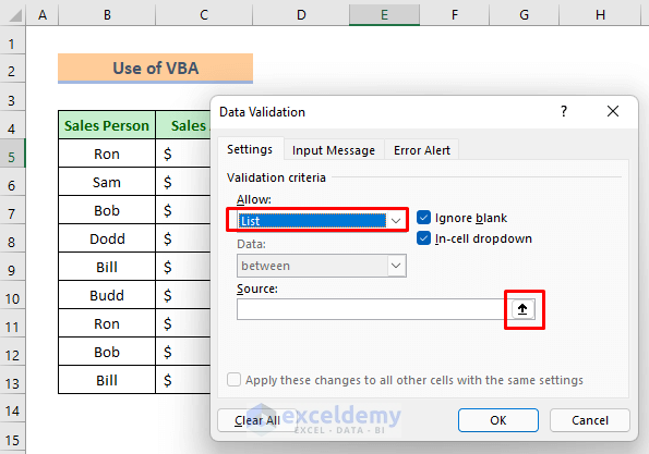
A dialog box will appear.

• Select List from the Allow bar.
• Press the Open icon from the Source bar.

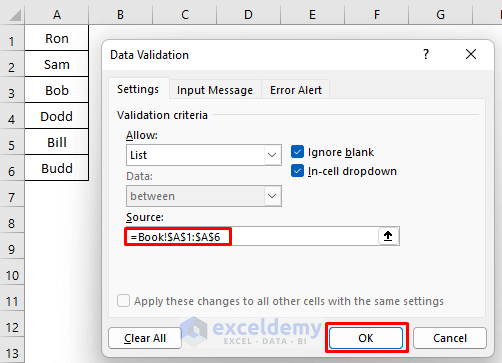
• Go to your new sheet and select the unique names.
• Press OK

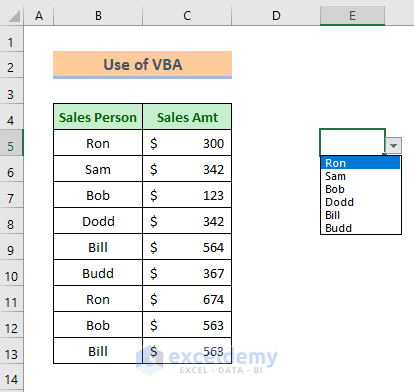
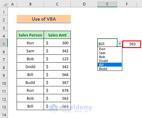
There’s a down arrow sign on cell E5’s right side. By clicking it you can select any name. That will save us time because we won’t need to type the names every time.

Now we’ll make a new function named LastItemLookup with Excel VBA.

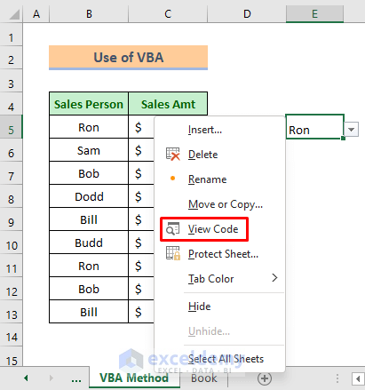
• Right-click your mouse on the sheet name.
• Select View Code from the context menu.

A VBA window will open up.

• Enter the code given below:

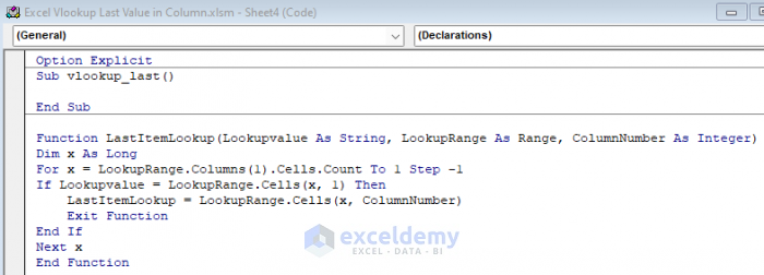
Option Explicit
Sub vlookup_last()
End Sub
Function LastItemLookup(Lookupvalue As String, LookupRange As Range, ColumnNumber As Integer)
Dim x As Long
For x = LookupRange.Columns(1).Cells.Count To 1 Step -1
If Lookupvalue = LookupRange.Cells(x, 1) Then
    LastItemLookup = LookupRange.Cells(x, ColumnNumber)
    Exit Function
End If
Next x
End Function

• Press the Play button to run the codes.

A dialog box named Macros will appear.

• Click Run.

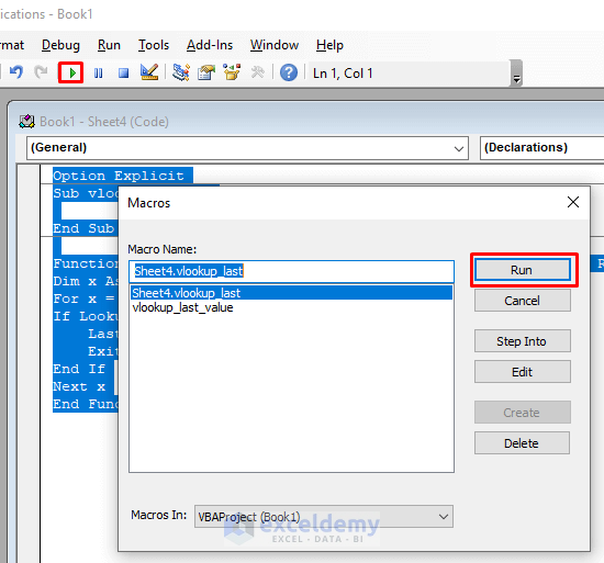
Our new function is ready now.

• Return to your worksheet.
• Activate Cell F5.
• Enter the formula given below:

Press Enter to get the last occurrence for Ron.

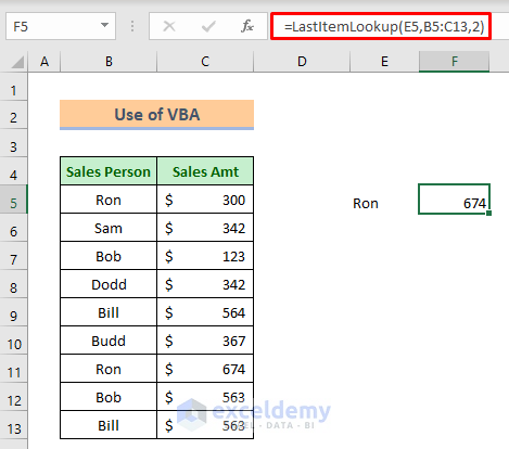
Now when you choose any salesman’s name then you will get his corresponding last occurrence value.

Download Practice Book

Related Articles

• How to Use VLOOKUP with Two Lookup Values in Excel
• How to Apply Double VLOOKUP in Excel?
• How to Use VLOOKUP Function with Exact Match in Excel
• How to Find Second Match with VLOOKUP in Excel
• VLOOKUP and Return All Matches in Excel
• VLOOKUP Fuzzy Match in Excel
• How to Use VLOOKUP to Search Text in Excel
• How to Apply VLOOKUP by Date in Excel
• Return the Highest Value Using VLOOKUP Function in Excel
• VLOOKUP with Numbers in Excel

<< Go Back to VLOOKUP a Range | Excel VLOOKUP Function | Excel Functions | Learn Excel