How to Find the Second Match with VLOOKUP in Excel (2 Methods)

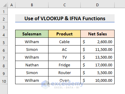
Dataset Overview

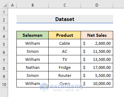
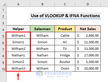
We’ll use a sample dataset that represents the Salesman, Product, and Net Sales of a company.

Introduction to Excel VLOOKUP Function

The VLOOKUP function allows you to search for a specific value in the leftmost column of a given table and retrieve a corresponding value from another column. Let’s break down its syntax:

• Syntax

=VLOOKUP(lookup_value, table_array, col_index_num, [range_lookup])

• lookup_value : The value you want to find in the leftmost column.
• table_array : The table where you’ll search for the lookup value (leftmost column).
• col_index_num : The column number from which you want to retrieve a value.
• [range_lookup]: Optional parameter that specifies whether an exact or partial match is required (0 for exact match, 1 for partial match).

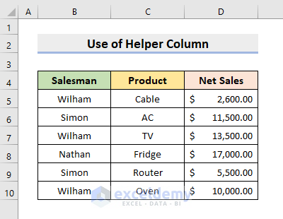
Method 1 – Using a Helper Column

STEPS

• Create a helper column (A5) to find the second match using the following formula:

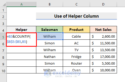
This formula generates a unique lookup value by combining the Salesman name (in cell B5) with the count of occurrences in the helper column.

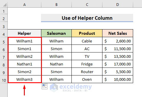
• Press Enter and use the AutoFill this formula down the column.

• To find the Net Sales of Wilham2, enter the following VLOOKUP formula in Cell G5:

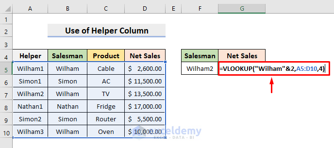
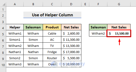
This formula looks for Wilham2 in the helper column and returns the corresponding value from the 4th column (Net Sales) in the range A5:D10.

• Press Enter to get the result.

Read More: How to Use VLOOKUP to Search Text in Excel

Method 2 – Excel VLOOKUP & IFNA Functions

STEPS

• Create the same Helper column as in Method 1.
• Select cell A5 and enter the formula:

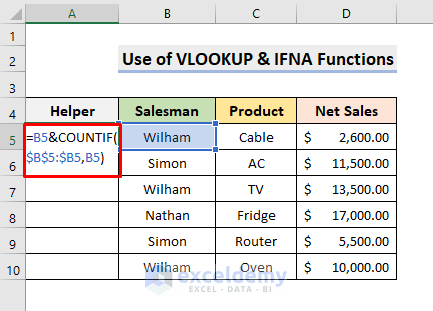
This formula generates a unique lookup value by combining the Salesman name (in cell B5) with the count of occurrences in the helper column.

• Press Enter and use the AutoFill this formula down the column.

• To find the Net Sales of Wilham2, enter this formula in cell G5:

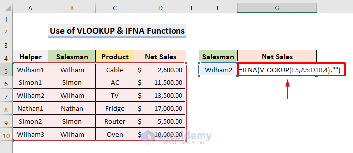
The IFNA function ensures that if no value is found, it returns a blank cell.

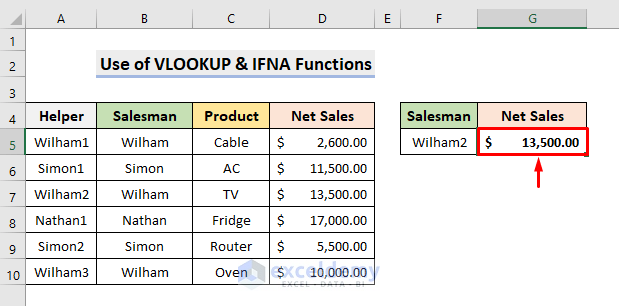
• Press Enter to get the result.

How Does the Formula Work?

➤ VLOOKUP(F5, A5:D10,4)

This part of the formula looks for the F5 cell value in the range A5:D10 and it returns the value present in the 4th column.

➤ IFNA(VLOOKUP(F5,A5:D10,4),””)

This part of the formula will just return the result of VLOOKUP(F5, A5:D10,4), but it’ll return a blank cell if there is no value available.

Read More: How to Apply Double VLOOKUP in Excel

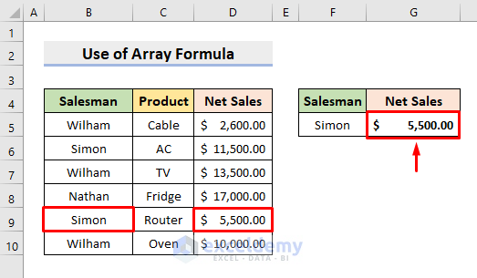
Alternative Approach: Array Formula

STEPS

• To find the Net Sales of Simon2, enter the following array formula in cell G5:

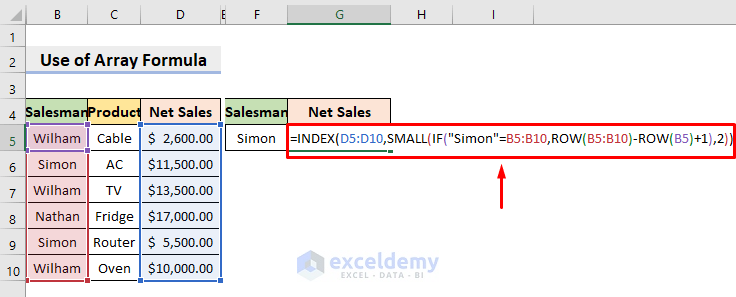
• Press Enter to get the result.

How Does the Formula Work?

• ROW(B5:B10) returns the row numbers of the cells.
• The logical test checks if Simon matches the Salesman names.
• SMALL(…, 2) retrieves the second smallest numeric value.
• INDEX(D5:D10, …) returns the desired value from the Net Sales column.

Read More: How to Use VLOOKUP Function with Exact Match in Excel

Download Practice Workbook

You can download the practice workbook from here:

Related Articles

• How to Use VLOOKUP with Two Lookup Values in Excel
• VLOOKUP and Return All Matches in Excel
• VLOOKUP Fuzzy Match in Excel
• Excel VLOOKUP to Find Last Value in Column
• How to Apply VLOOKUP by Date in Excel
• Return the Highest Value Using VLOOKUP Function in Excel
• VLOOKUP with Numbers in Excel

<< Go Back to VLOOKUP a Range | Excel VLOOKUP Function | Excel Functions | Learn Excel