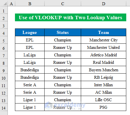
We have a table containing the roll of honor for the few major European football leagues. Using this dataset, we will VLOOKUP with two lookup values.
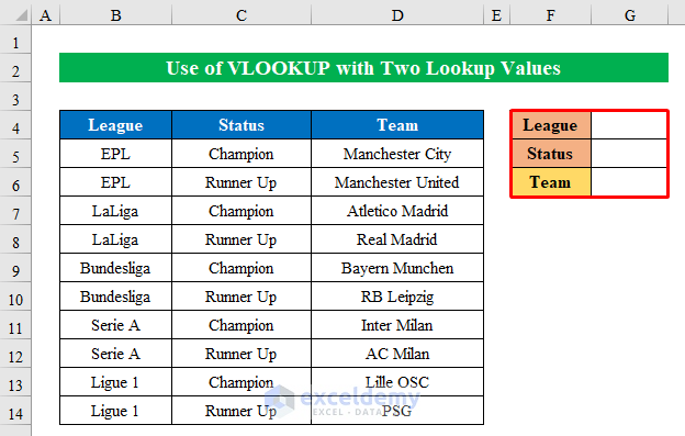
The league name and status will be provided as lookup values to find the team name, which are put in a smaller table to the side.
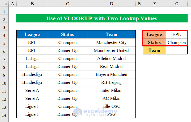
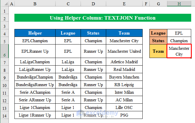
We have set EPL and Champion as the lookup League and Status values, respectively.
Method 1 – Inserting a Helper Column to Use VLOOKUP with Two Lookup Values in Excel
You may need to use a helper column for using two values within VLOOKUP.
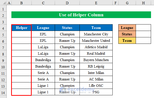
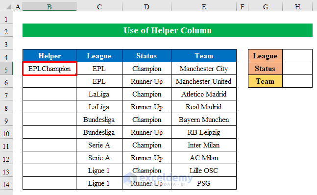
- The value of the Helper column will be the concatenation of the two lookup values corresponding to the data table.
- Here’s the formula you can use to make each cell in the helper column.
=C5&D5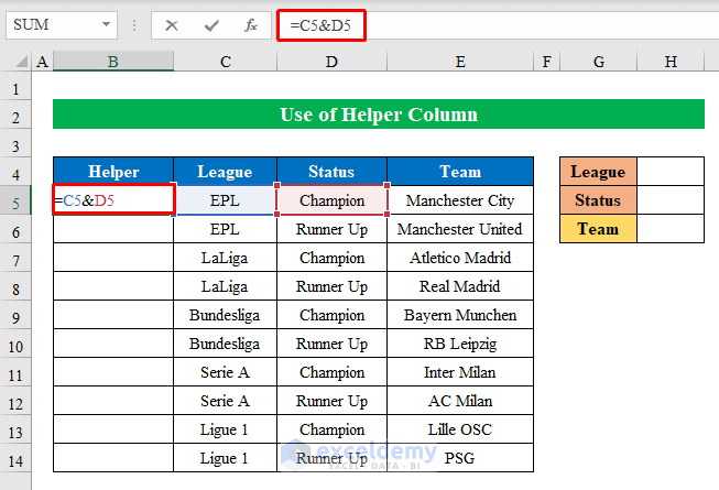
- C5 and D5 are the cell references for League and Status values respectively. This will join them together.
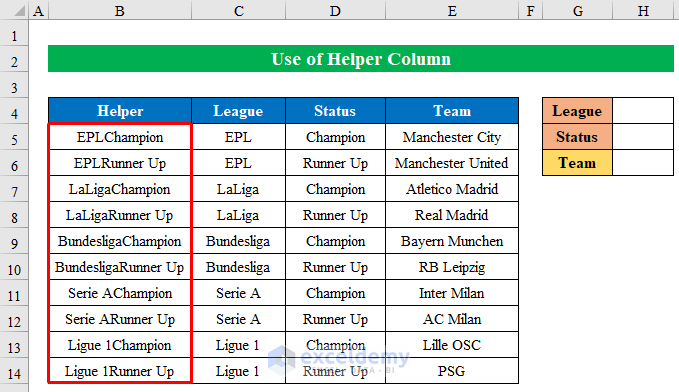
- Fill the rest of the rows for the Helper column.
Read More: 10 Best Practices with VLOOKUP in Excel
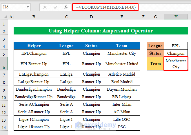
Case 1.1 – Concatenate with Ampersand
Steps:
- Choose the result cell H6 and insert the following:
=VLOOKUP(H4&H5,B5:E14,4,0)We have inserted the lookup values by joining them together using the ampersand sign. B5:E14 is the lookup range. Make sure the lookup value can be found in the very first column of this lookup_array.
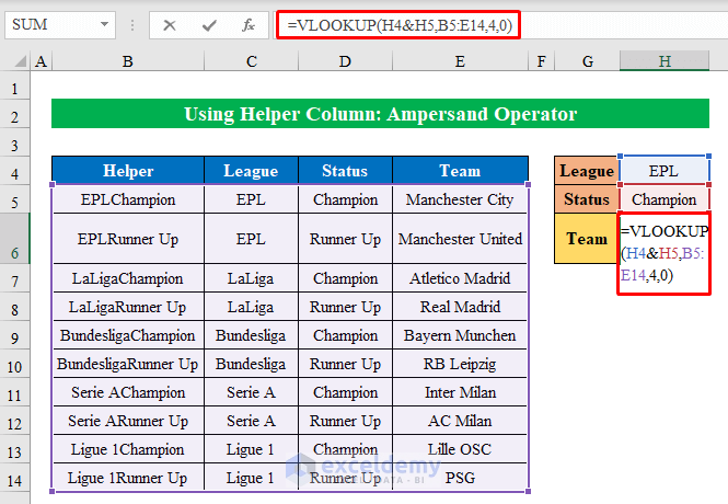
- Hit Enter to get the result.
Read More: 7 Practical Examples of VLOOKUP Function in Excel
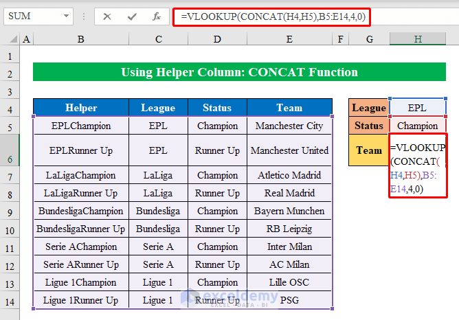
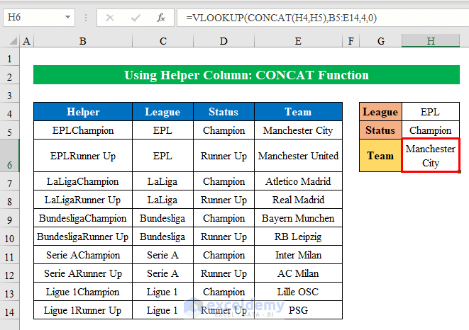
Case 1.2 – Concatenate with the CONCAT Function
Steps:
- Insert the following formula in H6.
=VLOOKUP(CONCAT(H4,H5),B5:E14,4,0)The CONCAT function joins the two values and then the rest of the mechanism will be the same. We will get the result (the team name depending on the criteria).
- Click Enter to get the output.
Case 1.3 – Concatenate with the TEXTJOIN Function
Steps:
- Use the following function in H6.
=VLOOKUP(TEXTJOIN(,TRUE,H4,H5),B5:E14,4,0)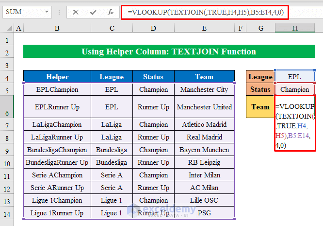
- Hit the Enter key to get the final output.
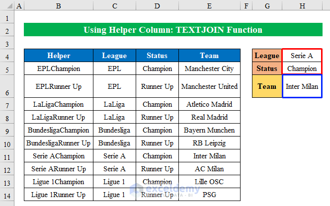
- If we change the inputs from the “League” and “Status” sections, the output will be changed according to the given conditions.
Read More: How to Apply Double VLOOKUP in Excel
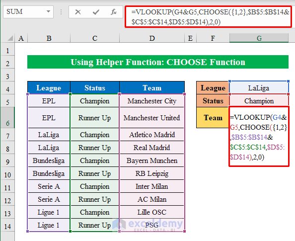
Method 2 – Combining VLOOKUP with the CHOOSE Function for Two Lookup Values
Steps:
- Choose cell G6 and insert the following formula in the cell:
=VLOOKUP(G4&G5,CHOOSE({1,2},$B$5:$B$14&$C$5:$C$14,$D$5:$D$14),2,0)The CHOOSE function returns a value from a list using a given position or index. The CHOOSE portion of this formula works as a virtual helper table. We have used 1 and 2 (within the curly braces) as the index number. We concatenated the League and Status columns together, which will be the first column of our virtual table. We have inserted the Team column in the value2 field, which will be the virtual table’s second column. This table becomes the lookup_array for the VLOOKUP. Since our desired result would be found at the second column from the virtual table, we have used 2 as the column_number.
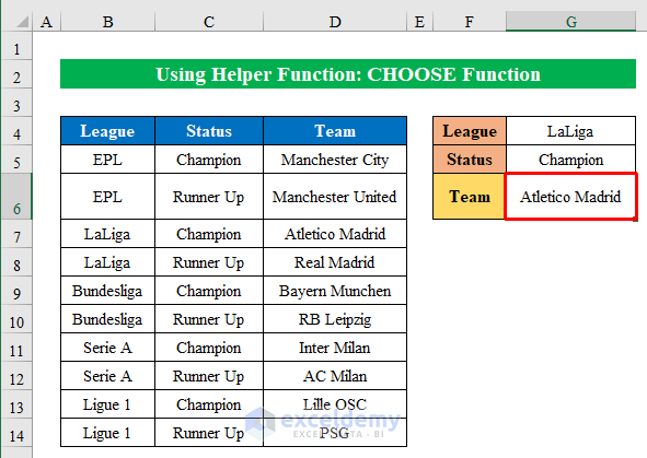
- Hit Enter to get the final output.
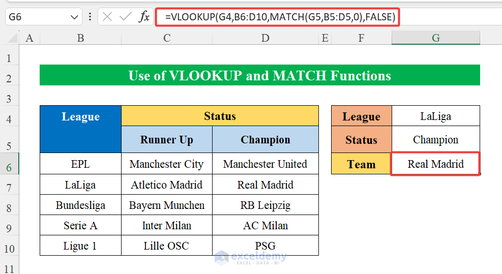
Method 3 – Using the MATCH Function with VLOOKUP for Two Lookup Values in Excel
Steps:
- Select cell G6 and enter the formula:
=VLOOKUP(G4,B6:D10,MATCH(G5,B5:D5,0),FALSE)The only lookup values are in Column B as League and Row C6: D10 as the name of the Champion team and the Runner Up team. G4 is the first lookup value and G5 is the second lookup value.
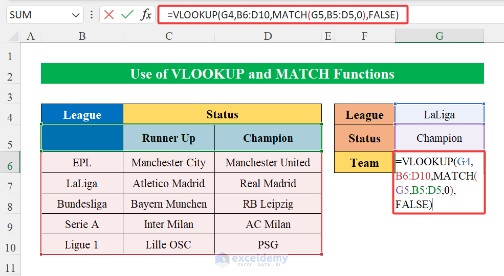
- Hit Enter.
Alternative – Combining INDEX and MATCH Functions for Two Lookup Values
Steps:
- Select G6 and apply the formula from below:
=INDEX(D5:D14, MATCH(1, (G4=B5:B14) * (G5=C5:C14), 0))The INDEX-MATCH function works as a two-way lookup. The MATCH function will look for values given in cells (G4) and (G5) from the range (B5:C5:C14). The INDEX function will retrieve the value at the given location from a range (D5:D14).
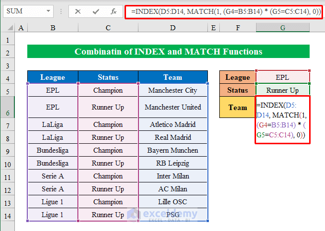
- Hit Enter.

Download the Practice Workbook
Related Articles
- How to Use VLOOKUP Function with Exact Match in Excel
- How to Find Second Match with VLOOKUP in Excel
- VLOOKUP and Return All Matches in Excel
- VLOOKUP Fuzzy Match in Excel
- Excel VLOOKUP to Find Last Value in Column
- How to Use VLOOKUP to Search Text in Excel
- How to Apply VLOOKUP by Date in Excel
- Return the Highest Value Using VLOOKUP Function in Excel
- VLOOKUP with Numbers in Excel
<< Go Back to VLOOKUP Multiple Values | Excel VLOOKUP Function | Excel Functions | Learn Excel
Get FREE Advanced Excel Exercises with Solutions!

Fascinating article. Very inventive combination of functions. One problem, option 3 does not work as posted. If you run the function it will return the first entry that it finds rather than whichever one you are trying to capture. There is no way to indicate whether you want the champion or the runner-up.
Hello Rick Howard, Thank you for your query. Therefore, method 3 is updated in the article. Now you may find any champion team or any runner Up team of any random League using The VLOOKUP function and the MATCH function.