Method 1 – Using COUNTIF and VLOOKUP Functions to Vlookup Multiple Values
- Select cell C5 to add the salesperson’s number.
=D5&COUNTIF($D$5:D5,D5)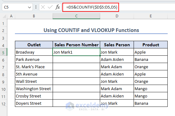
- Select cell C16 to solve this issue.
=VLOOKUP(C14&C15,$C$5:$E$12,3,0)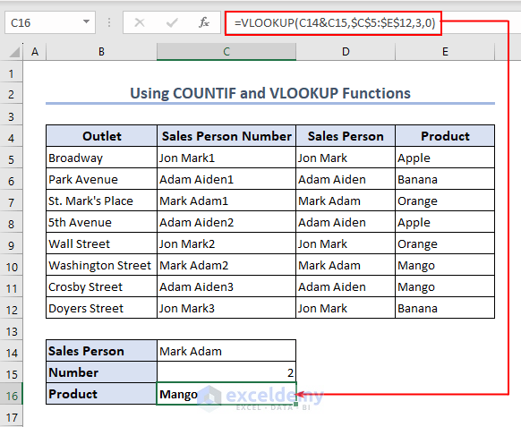
Method 2: Applying the VLOOKUP Function with Helper Column
- Select cell C5 to add the helper column and enter the formula below.
=D5&""&E5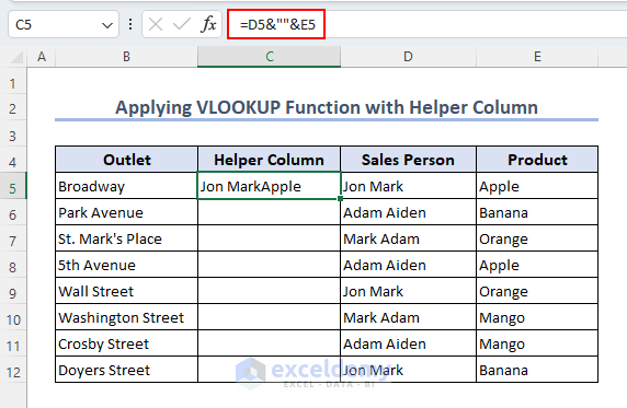
- Enter the value of any helper column in cell C14 and look up the product value of the helper.
- Select cell C15 and enter the formula to extract the product’s value.
=VLOOKUP(C14,$C$5:$E$12,3,0)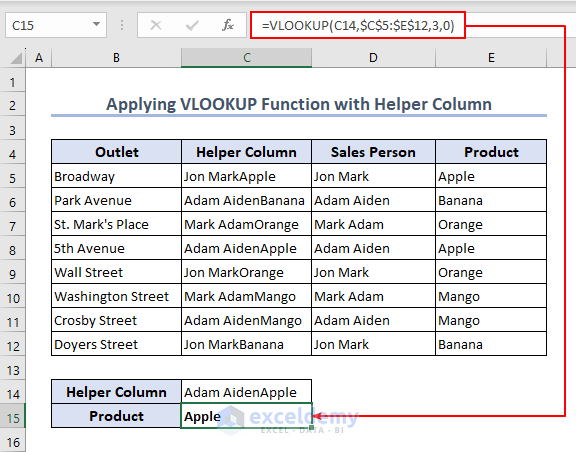
Method 3 – Using the VLOOKUP Function in Both Rows and Columns
- Select cell C17 to enter the formula and extract the value from rows and columns.
=VLOOKUP(C15,B6:H13, MATCH(C16, B5:H5, 0), FALSE)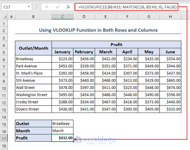
Formula Breakdown
MATCH(C16, B5:H5, 0)
- This part of the formula returns the values as true in cell C16 if there is a match in the range B5:H5.
VLOOKUP(C15,B6:H13, MATCH(C16, B5:H5, 0), FALSE)
- The formula will return the value from March if the value matches the range B6:H13.
Read More: How to Use Excel VLOOKUP to Return Multiple Values Vertically
How to Vlookup Multiple Values Without VLOOKUP Function in Excel: 5 Methods
Method 1 – Vlookup Multiple Values in a Column
STEPS:
- Select cell F5 to enter the formula and extract multiple values in a column.
=IFERROR(INDEX($D$5:$D$12, SMALL(IF(F$4=$C$5:$C$12, ROW($D$5:$D$12)-4,""), ROW()-4)),"")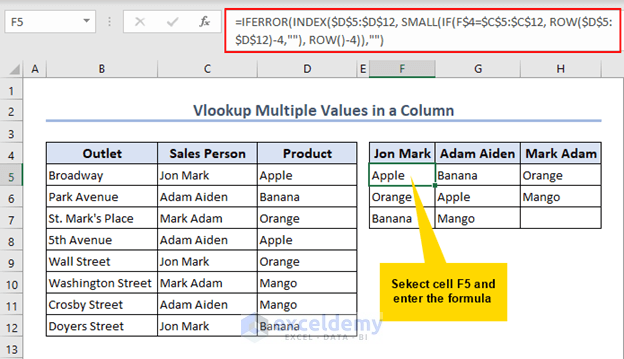
Formula Breakdown
ROW($D$5:$D$12)-4,””), ROW()-4)
- This part will return the value on the 5th row and 5th column from the dataset regarding the range D5:D12.
IF(F$4=$C$5:$C$12, ROW($D$5:$D$12)-4,””), ROW()-4))
- This part will Extract the value from the range C5:C12 regarding cell F4.
SMALL(IF(F$4=$C$5:$C$12, ROW($D$5:$D$12)-4,””), ROW()-4)
- The SMALL function will extract the smallest value from the array using the IF function.
(INDEX($D$5:$D$12, SMALL(IF(F$4=$C$5:$C$12, ROW($D$5:$D$12)-4,””), ROW()-4)),””)
- This part will return the formula as an array if the lookup values match the function; otherwise, it will return #ERROR.
IFERROR(INDEX($D$5:$D$12, SMALL(IF(F$4=$C$5:$C$12, ROW($D$5:$D$12)-4,””), ROW()-4)),””)
- The formula will return the value if the lookup value matches the formula; otherwise, it will return blank.
Read More: VLOOKUP to Return Multiple Values Horizontally in Excel
Method 2 – Vlookup Multiple Values in a Row
- Here, we will look up multiple values in cell G5 using the same process. But instead of using the ROW function both times, here we will use the COLUMN function to look up multiple values in a row.
=IFERROR(INDEX($D$5:$D$12, SMALL(IF($F5=$C$5:$C$12, ROW($D$5:$D$12)-4,""), COLUMN()-6)),"")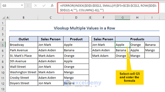
Read More: How to Use VLOOKUP Function on Multiple Rows in Excel
Method 3 – Vlookup Multiple Values for Multiple Criteria
This method will complete the process for multiple criteria in cell H5. Here, we will use the same functions as earlier.
=IFERROR(INDEX($D$5:$D$12, SMALL(IF(1=((--($F$6=$C$5:$C$12)) * (--($G$6=$B$5:$B$12))), ROW($D$5:$D$12)-4,""), ROW()-4)),"")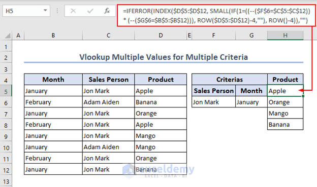
Method 4 – Applying INDEX and MATCH Functions to Vlookup Multiple Values
We will use the INDEX and MATCH functions to complete the process in this method.
- Select cell C16 and enter the formula below:
=INDEX(D5:D12, MATCH(1, (C14=C5:C12) * (C15=B5:B12), 0))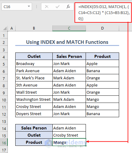
Formula Breakdown
MATCH(1, (C14=C5:C12) * (C15=B5:B12)
- This part will return the value as true if both ranges C5:C12 and B5:B12 return the value from C14 and C15.
INDEX(D5:D12, MATCH(1, (C14=C5:C12) * (C15=B5:B12), 0))
- The formula will return the value if the index range matches the formula; otherwise, it will return N/A.
Method 5 – Using VBA Macro to Vlookup Multiple Values
In this method, we will use a VBA Macro to solve this issue in Excel.
- Go to Developer >> Visual Basic and open the VBA window.
- Select Insert >> Module to enter the code and execute the process.
Code
Sub VLookupSalesData()

Dim LookupRange As Range

Dim Criteria As String

Dim Result() As Variant

Dim FoundRow As Range

Dim i As Long

Set LookupRange = Range("B5:E12")

Criteria = Range("G5").Value

For Each FoundRow In LookupRange.Columns(2).Cells

If FoundRow.Value = Criteria Then

ReDim Preserve Result(i)

Result(i) = FoundRow.Offset(0, 1).Value

i = i + 1

End If

Next FoundRow

If i > 0 Then

Range("F9").Resize(i).Value = WorksheetFunction.Trans_

pose (Result)

Else

Range("F9").Value = "Not found"

End If

End Sub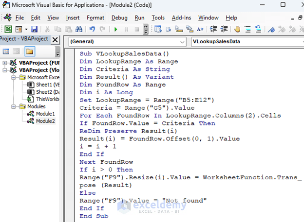
Code Breakdown
Sub VLookupSalesData()

Dim LookupRange As Range

Dim Criteria As String

Dim Result() As Variant

Dim FoundRow As Range

Dim i As Long- This code is named as VLookupSalesData where the lookup range and FoundRow are declared as Range, Criteria is declared as String, Result is declared as an array and i as Long.
Set LookupRange = Range("B5:E12")

Criteria = Range("G5").Value

For Each FoundRow In LookupRange.Columns(2).Cells

If FoundRow.Value = Criteria Then

ReDim Preserve Result(i)

Result(i) = FoundRow.Offset(0, 1).Value

i = i + 1- Here, the lookup range is B5:B12, and the lookup value is cell G5. The code will start from column B and find the value from column B. If the criteria match, we will execute the IF. After that, we will resize the result value and assign it to one column right of the current column.
End If

Next FoundRow

If i > 0 Then

Range("F9").Resize(i).Value = WorksheetFunction.Trans_

pose (Result)

Else

Range("F9").Value = "Not found"

End If

End Sub
End the IF statement if the value matches the function and move on to the loop where the value of i is greater than Zero (0). Then, the result value in cell F9 is resized and the result value is transposed. Lastly, assign the code in cell F9 as “Not Found” and complete the process.
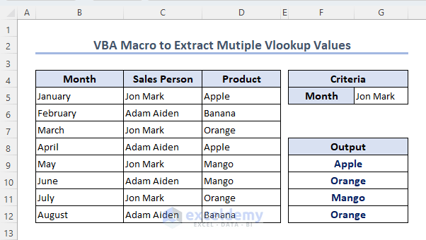
- Here is the final output in the Output
How to Use Nested VLOOKUP Function to Vlookup Multiple Values in Excel
Here, we will use the nested VLOOKUP function to execute the process in Excel in cell I5.
=VLOOKUP(VLOOKUP(H5, $B$5:$C$12, 2, FALSE), $E$5:$F$12, 2, FALSE)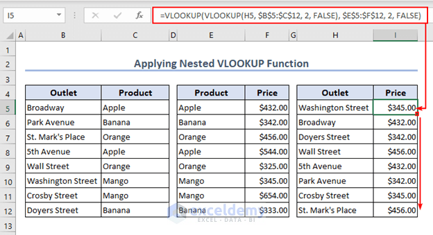
Formula Breakdown
VLOOKUP(H5, $B$5:$C$12, 2, FALSE)
- In this part, the function will return the value of the Outlet if the lookup range matches the lookup value.
VLOOKUP(VLOOKUP(H5, $B$5:$C$12, 2, FALSE), $E$5:$F$12, 2, FALSE)
- Here, the output of the VLOOKUP function will be used as the lookup range in the second VLOOKUP function, which will return a value if the formula matches the lookup range.
Things to Remember
- The VLOOKUP function does not by default return multiple values. So, as already shown, we need to use another part to look up multiple values.
- Always set up the correct range while using the function, and try to use the absolute range using the ($)
Download the Practice Workbook
You may download the below workbook for practice.
VLOOKUP Multiple Values: Knowledge Hub
- How to VLOOKUP Multiple Values in One Cell in Excel
- Find Max of Multiple Values by Using VLOOKUP Function in Excel
- How to Vlookup and Return Multiple Values in Drop Down List
- Excel VLOOKUP to Return Multiple Values in One Cell Separated by Comma
- VLOOKUP with Multiple Matches in Excel
<< Go Back to Advanced VLOOKUP | Excel VLOOKUP Function | Excel Functions | Learn Excel
Get FREE Advanced Excel Exercises with Solutions!
