Method 1 – Use of INDEX, SMALL, and IF Functions to VLOOKUP and Return Corresponding Values Horizontally
Step 1:
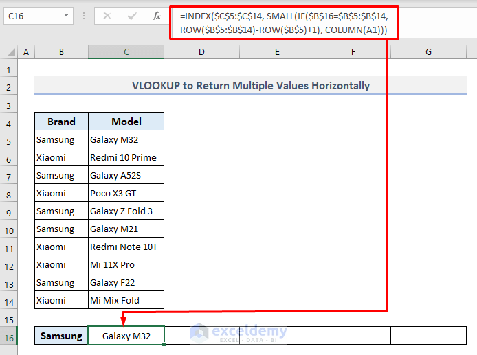
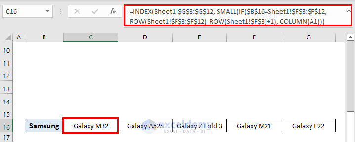
➤ The required formula in cell C16 will be:
=INDEX($C$5:$C$14, SMALL(IF($B$16=$B$5:$B$14,ROW($B$5:$B$14)-ROW($B$5)+1), COLUMN(A1)))➤ After pressing Enter, you’ll get the first model name of Samsung from the table.
Step 2:
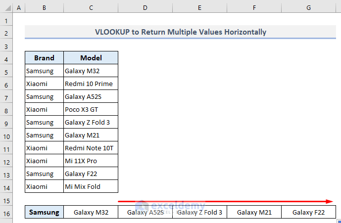
➤ Use Fill Handle from cell C16 and drag it rightward along Row 16 until a #NUM error appears.
➤ Skip the first #NUM error and stop auto-filling before that cell containing the error.
You’ll be shown all the model names of Samsung smartphones horizontally in the table.
How Does the Formula Work?
- ROW($B$5:$B$14)-ROW($B$5)+1: This part is assigned to the second argument ([value_if_true]) of the IF function. It defines the row number of all data available in the range of cells B5:B14 and returns the following array:
{1;2;3;4;5;6;7;8;9;10}
- IF($B$16=$B$5:$B$14, ROW($B$5:$B$14)-ROW($B$5)+1): This part of the formula matches the criteria for Samsung devices only. If a match is found, the formula will return the perspective row number; otherwise, it’ll return FALSE. So, the overall return array from this formula will be:
{1;FALSE;3;FALSE;5;6;FALSE;FALSE;9;FALSE}
- SMALL(IF($B$16=$B$5:$B$14, ROW($B$5:$B$14)-ROW($B$5)+1), COLUMN(A1)): The SMALL function here extracts the lowest or smallest row number found from the previous step, and it’ll be defined as the second argument (row_num) of the INDEX function.
- The entire and combined formula extracts the first model name of Samsung devices from Column C.
Method 2 – VLOOKUP and Return Multiple Values Horizontally from a Sequence of Data in Excel
Step 1:
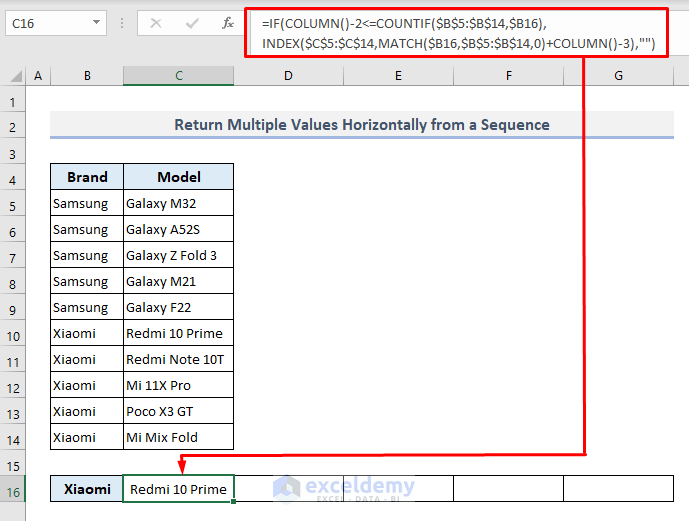
➤ In the output Cell C16, the required formula will be:
=IF(COLUMN()-2<=COUNTIF($B$5:$B$14,$B16), INDEX($C$5:$C$14,MATCH($B16,$B$5:$B$14,0)+COLUMN()-3),"")➤ Press Enter, and you’ll be displayed the first smartphone model name of Xiaomi immediately.
Step 2:
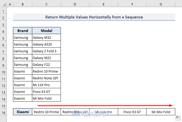
➤ Use Fill Handle to autofill rightward along Row 16 until a blank cell appears.
You’ll be displayed all the model names of the selected brand only like in the screenshot below.
How Does the Formula Work?
- MATCH($B16,$B$5:$B$14,0): The MATCH function inside the INDEX function returns the first-row cell number containing the name- Xiaomi.
- MATCH($B16,$B$5:$B$14,0)+COLUMN()-3: This part is the second argument of the INDEX function, which defines the row number where the first resultant data will be looked for.
- INDEX($C$5:$C$14, MATCH($B16,$B$5:$B$14,0)+COLUMN()-3): This part is the second argument of the IF function ([value_if_TRUE]), which extracts the first output data based on the row number found in the previous step.
- The IF function will return a blank cell if no match is found.
Note: To return data with this formula properly, you must initiate the table from Column B where Column B will represent the criteria and Column C will have the output data. You also have to define the selected criteria in Column B under or above the table as I’ve shown in Cell B16.
Download Practice Workbook
You can download the Excel workbook that we’ve used to prepare this article.
Related Articles
- How to Vlookup and Return Multiple Values in Drop Down List
- How to Use VLOOKUP Function on Multiple Rows in Excel
- How to VLOOKUP Multiple Values in One Cell in Excel
- Excel VLOOKUP to Return Multiple Values in One Cell Separated by Comma
<< Go Back to VLOOKUP Multiple Values | Excel VLOOKUP Function | Excel Functions | Learn Excel
Get FREE Advanced Excel Exercises with Solutions!

Hi, thanks for this post, I solved my problem on excel with this post. Thank you so much
Hi Michael,
Thanks for your feedback!
If you move the main lookup table to a new sheet this formulae doesn’t work
Hi KRISB,
I hope you are doing well.
If you copy the table and paste it somewhere else, then Excel will not adjust cell references according to the move.
The formula should work fine if you cut the table and paste it into another sheet.
For instance, I have cut the table and pasted it into “sheet1”. Then Excel automatically modifies the formula. See the image for better clarification.
The table was shifted in “sheet1”
in this exapmle only two brands are showing, suppose if i have mothen than 50 brands and i want to drag this formula vertially for all brands shall it work?
Hello SUNZEEV,
Thank you for your comment. Here, we are providing two revised formulas to meet your requirements.
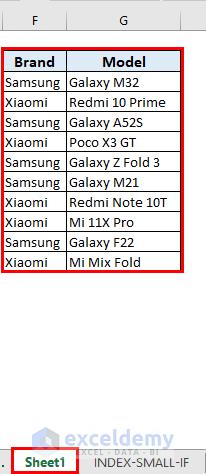
For simplicity, we have modified the dataset with two additional Company names.
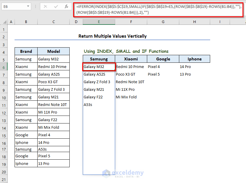
To get all the device names for each company, write the following formula in E6 and press Enter.
=IFERROR(INDEX($B$5:$C$19,SMALL(IF($B$5:$B$19=E5,(ROW($B$5:$B$19)-ROWS(B1:B4)),""),(ROW($B$5:$B$19)-ROWS(B1:B4))),2),"")You will get all the results of Samsung at once.
Now, drag the E6 cell to the right to H6 cell. You will get your desired results.
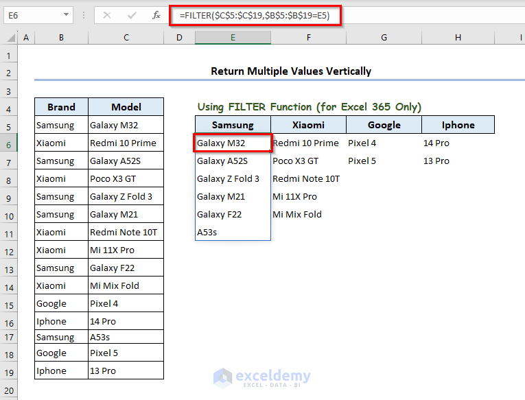
Another way is to use the FILTER function. For this method, write the following formula in E6 and press Enter.
=FILTER(C5:C19,B5:B19=E5)Now, drag the E6 cell to the right to the H6 cell. You will get your desired results. The FILTER function is available on Excel 365 only.
You can download the workbook from the link below.
Answer.xlsx
We hope these methods will satisfy your queries. If you have further questions, you are always welcome.
Regards,
Sourav
ExcelDemy.