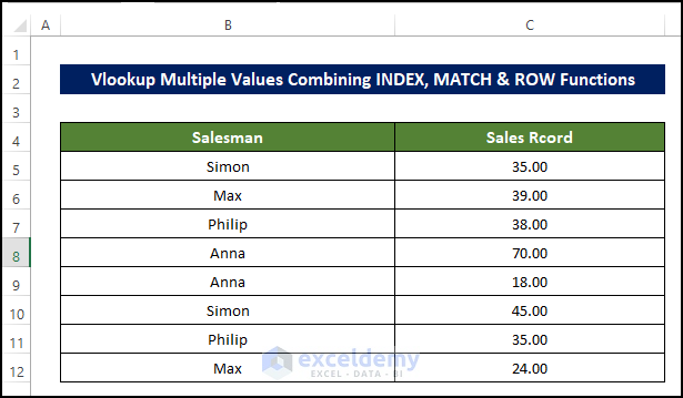
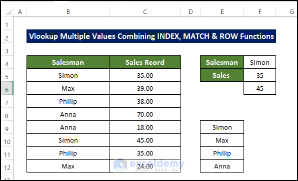
Method 1 – Vlookup Multiple Values Combining the INDEX, MATCH & ROW Functions
Steps
This is the sample dataset..
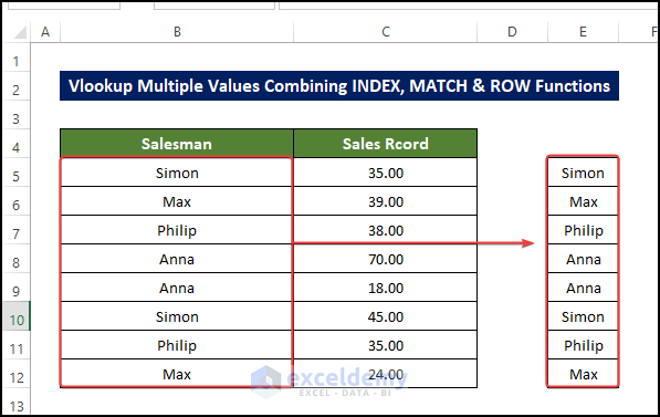
- To create a drop-down list, copy the salesperson’s name to the right side of the sheet. Here, E5:E12.
- Select E5:E12 and go to Data tab > Data Tools> Remove duplicate.
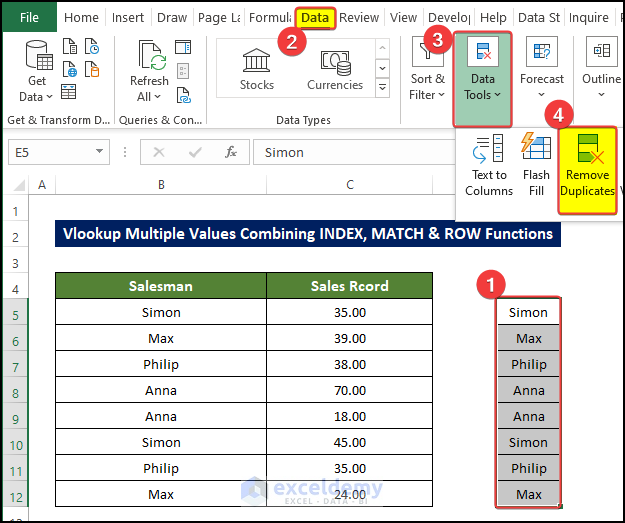
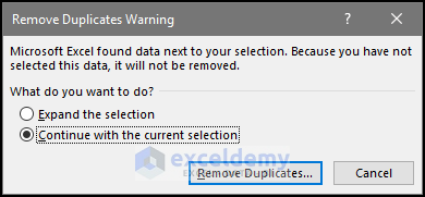
- In the warning window, select Continue with the current selection.
- Click Remove Duplicates.
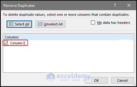
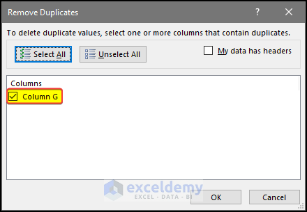
- Check Column E.
- Click OK.
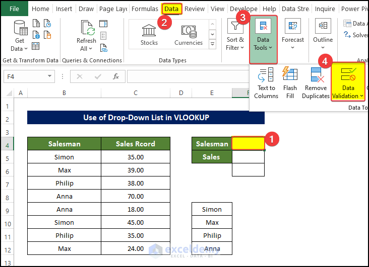
- Arrange the cell as shown below.
- Select F4 and go to Data tab > Data tools > Data Validation.
- Go to the Settings tab.
- Select List.
- Select E9:E12 in Source.
- Click OK.
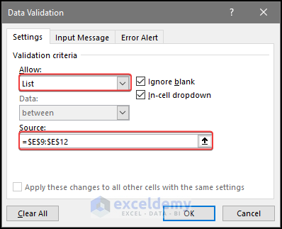
The drop-down list is created.
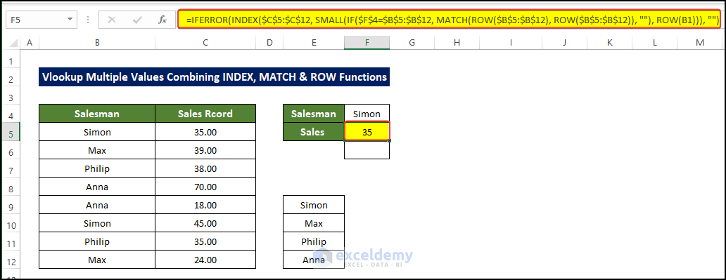
- Select F5 and enter the following formula:
=IFERROR(INDEX($C$5:$C$12, SMALL(IF($F$4=$B$5:$B$12, MATCH(ROW($B$5:$B$12), ROW($B$5:$B$12)), ""), ROW(B1))), "")
It will return Simon’s sales value.
Formula Breakdown
ROW($B$5:$B$12)
returns the row number of the range of cells in array format.
MATCH(ROW($B$5:$B$12), ROW($B$5:$B$12))
matches the location of the row array values in the output of the ROW output. The output is 1,2,3,4,5,6,7,8.: the serial of the matched value.
IF($F$4=$B$5:$B$12, MATCH(ROW($B$5:$B$12), ROW($B$5:$B$12)), “”)
The IF function enters a loop. If any value in B5:B13 is equal to the F4, the MATCH function will be executed. The matched cells serial in B5:B13 are determined through the MATCH function. Here, F4 displays Simon. The if function searches for Simon in B5:B13. Simon is found in B5. In the MATCH function, B5 is in the 1st and 6th serial in the range of cells. It returns 1 and 6.
SMALL(IF($F$4=$B$5:$B$12, MATCH(ROW($B$5:$B$12), ROW($B$5:$B$12)), “”), ROW(B1))
The SMALL function gets the nth smallest value of the output in the previous section of the formula. Here the output of ROW(B1) is 1.
INDEX($C$5:$C$12, SMALL(IF($F$4=$B$5:$B$12, MATCH(ROW($B$5:$B$12), ROW($B$5:$B$12)), “”), ROW(B1)))
This portion extracts the cell value according to the serial returned by the previous part of the formula.
IFERROR(INDEX($C$5:$C$12, SMALL(IF($F$4=$B$5:$B$12, MATCH(ROW($B$5:$B$12), ROW($B$5:$B$12)), “”), ROW(B1))), “”)
This part avoids error values, replacing them with a “”(space).
- Drag down the Fill Handle to see the result in the rest of the cells.
- You will see all values related to Simon.
Read More: How to Use VLOOKUP Function on Multiple Rows in Excel
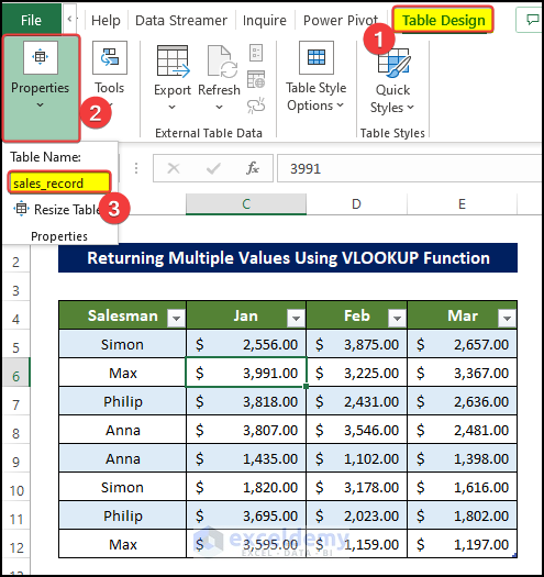
Method 2 – Return Multiple Values Using the VLOOKUP Function
Steps
- Create a table as shown below. Change its name to sales_record in the Table Design tab.
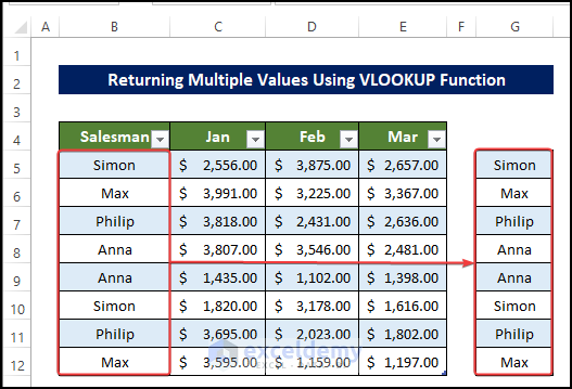
- To create a drop-down list, copy the salesperson’s name to the right side of the sheet. Here, E5:E12.
- Select E5:E12 and go to Data tab > Data Tools> Remove duplicate.
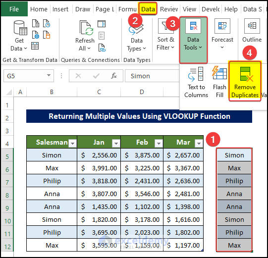
- Check Column E.
- Click OK.
- Arrange the cell as shown below.
- Select F4 and go to the Data tab > Data tools > Data Validation.
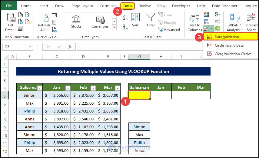
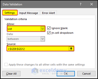
- Go to the Settings tab.
- Select List.
- Select E9:E12 in Source.
- Click OK.
The drop-down list is created.
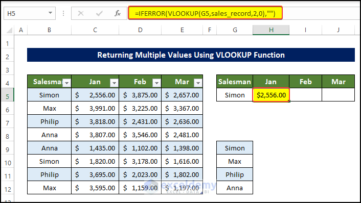
- Select F5 and enter the following formula:
=IFERROR(VLOOKUP(G5,sales_record,2,0),"")
Formula Breakdown
VLOOKUP(G5,sales_record,,0)
The VLOOKUP function looks for the location of the value in G5 in the Salesman column. If it finds the value, it will return the cell value in the 2-column offset, in the same row.
IFERROR(VLOOKUP(G5,sales_record,2,0),””)
This part avoids error values, replacing them with a “”(space).
- Select I5 and enter the following formula:
=IFERROR(VLOOKUP(G5,sales_record,3,0),"")
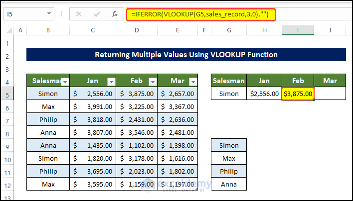
Formula Breakdown
VLOOKUP(G5,sales_record,3,0)
The VLOOKUP function looks for the location of the value in G5 in the Salesman column. If it finds the value, it will return the cell value in the 4-column offset, in the same row.
IFERROR(VLOOKUP(G5,sales_record,3,0),””)
This part avoids error values, replacing them with a “”(space).
- Select J5 and enter the following formula:
=IFERROR(VLOOKUP(G5,sales_record,4,0),"")
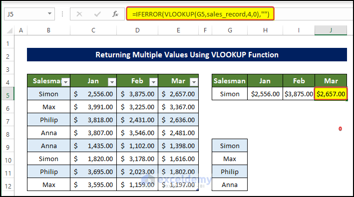
Formula Breakdown
VLOOKUP(G5,sales_record,4,0)
The VLOOKUP function looks for the location of the value in G5 in the Salesman column. If it finds the value, it will return the cell value in the 4-column offset, in the same row.
IFERROR(VLOOKUP(G5,sales_record,4,0),””)
This part avoids error values, replacing them with a “”(space).
Read More: How to Use Excel VLOOKUP to Return Multiple Values Vertically
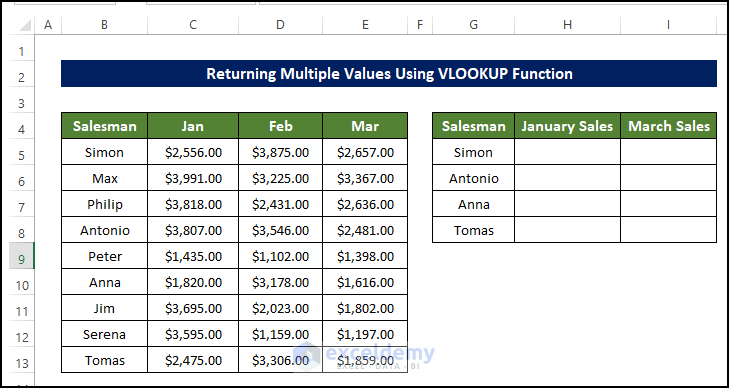
Can the VLOOKUP Function Return Multiple Values?
Yes, if the lookup value contains a range:
Steps
Consider the dataset below. To get the sales record of multiple salesmen:
- Select H5 and enter the following formula:
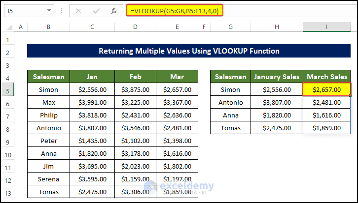
=VLOOKUP(G5:G8,B5:E13,2,0)
- All sales records in January are displayed in column H.
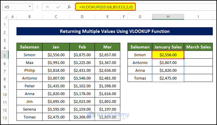
Note
The output is an array.
- To get the sales in March, select I5 and enter the following formula:
=VLOOKUP(G5:G8,B5:E13,4,0)
This is the output.
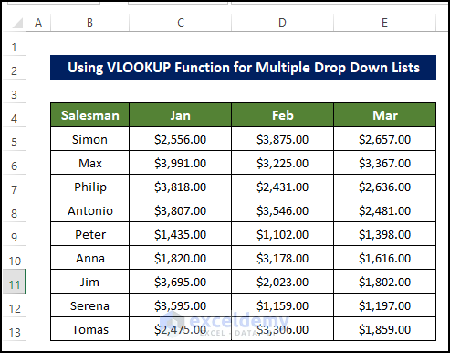
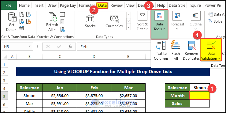
How to Use the VLOOKUP Function for Multiple Drop Down Lists in Excel
Steps
Create two separate drop-down lists in the dataset below:
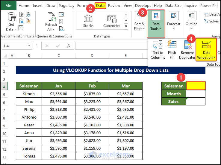
- To create the first drop-down list, select H4 and go to the Data tab > Data tools > Data Validation.
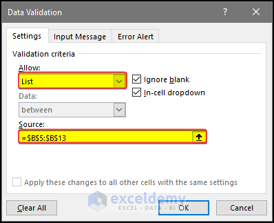
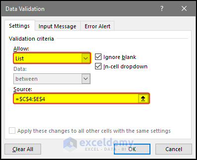
- Select Settings.
- Choose List.
- Select B5:B13 in Source.
- Click OK.
- To add the second drop-down list, select H5 and go to the Data tab > Data tools > Data Validation.
- Select Settings.
- Choose List.
- Select C4:E4 in Source.
- Click OK.
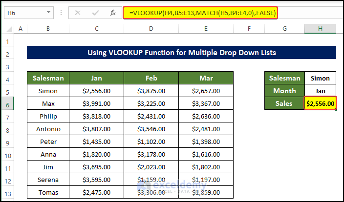
- Select H6 and enter the following formula:
=VLOOKUP(H4,B5:E13,MATCH(H5,B4:E4,0),FALSE)
Formula Breakdown
MATCH(H5,B4:E4,0)
gets the serial value in H5 in B4:E4. Here, the output is 2.
VLOOKUP(H4,B5:E13,MATCH(H5,B4:E4,0),FALSE)
looks for the value of H4 in B5:E13 and returns the value in the cell offset to the number returned in the MATCH function: 2.
Download Practice Workbook
Download this practice workbook.
Related Articles
- Excel VLOOKUP to Return Multiple Values in One Cell Separated by Comma
- How to VLOOKUP Multiple Values in One Cell in Excel
- VLOOKUP to Return Multiple Values Horizontally in Excel
- Find Max of Multiple Values by Using VLOOKUP Function in Excel
<< Go Back to VLOOKUP Multiple Values | Excel VLOOKUP Function | Excel Functions | Learn Excel
Get FREE Advanced Excel Exercises with Solutions!
