Looking for ways to know how to VLOOKUP to return min value from multiple hits? We can VLOOKUP to return min value in Excel using different functions. Here, you will find 4 ways to VLOOKUP to return min value from multiple hits.
Excel VLOOKUP Function to Return Min Value from Multiple Hits: 4 Ways
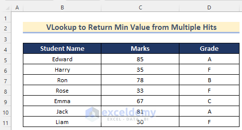
Here, we have a dataset containing the Student Name, Marks, and Grade of some students. Now, we will use this dataset to show you how to VLOOKUP to return min value from multiple hits.
1. Using MIN and VLOOKUP Functions to Return Min Value from Multiple Hits
In the first method, we will show you how to VLOOKUP to return min value from multiple hits using the MIN and VLOOKUP functions in Excel. The MIN function returns the minimum value in a range.
Hence, go through the steps given below to do it on your own dataset.
Steps:
- Firstly, select Cell B14.
- Then, insert the following formula.
=VLOOKUP(MIN($C$5:$C$11),$C$5:$D$11,{1,2},FALSE)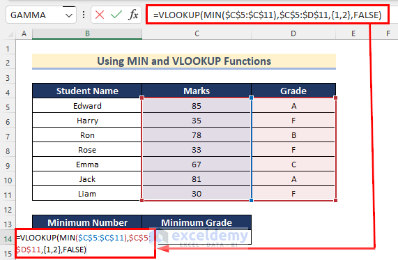
Here, in the formula, we inserted Cell range C5:C11 as number_1 in the MIN function to get the minimum value in the range. Then, in the VLOOKUP function, we set the result obtained from the MIN function as lookup_value, Cell range C5:D11 as table_array, 1 and 2 as col_index_num, and FALSE as range_lookup.
- After that, press ENTER to get the value of Minimum Number and Minimum Grade.

Read More: Find Max of Multiple Values by Using VLOOKUP Function in Excel
2. Applying SMALL Function with VLOOKUP Function to Return Min Value
We can also use the SMALL Function to VLOOKUP to return min value from multiple hits. The SMALL function returns the nth lowest or smallest value of a given range. Now, follow the steps given below to use this function along with the VLOOKUP function to VLOOKUP to return min value from multiple hits in your dataset.
Steps:
- Firstly, select Cell B14.
- Then, insert the following formula.
=VLOOKUP(SMALL(C5:C11,1),C5:D11,{1,2},FALSE)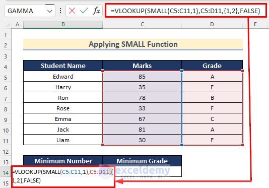
Here, in the formula, we inserted Cell range C5:C11 as an array and 1 as k (nth value) in the SMALL function to get the 1st minimum value in the range. Then, in the VLOOKUP function, we set the result obtained from the SMALL function as lookup_value, Cell range C5:D11 as table_array, 1 and 2 as col_index_num, and FALSE as range_lookup.
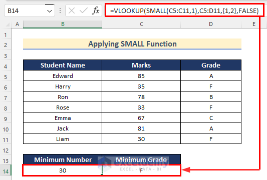
- After that, press ENTER to get the value of Minimum Number and Minimum Grade.
Read More: VLOOKUP to Return Multiple Values Horizontally in Excel
3. Use of VLOOKUP and MINA Functions to Return Min Value
Now, we will show you how to VLOOKUP to return min value from multiple hits using the MINA and VLOOKUP functions in Excel. The MINA function returns the smallest value in a range or list. Go through the steps given below to do it on your own dataset.
Steps:
- Firstly, select cell B14.
- Then, insert the following formula.
=VLOOKUP(MINA(C5:C11),$C$5:$D$11,{1,2},0)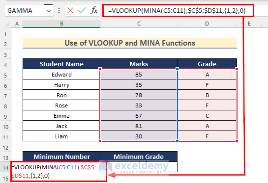
Here, in the formula, we inserted Cell range C5:C11 as value_1 in the MINA function to get the minimum value in the range. Then, in the VLOOKUP function, we set the result obtained from the MIN function as lookup_value, Cell range C5:D11 as table_array, 1 and 2 as col_index_num, and FALSE as range_lookup.
- After that, press ENTER to get the value of Minimum Number and Minimum Grade.

Read More: How to VLOOKUP and Return Multiple Values in Drop Down List
4. Return Min Value from Multiple Hits Based on Criteria in Excel
Moreover, we will show you how to VLOOKUP to return minimum value from multiple hits for any specific criteria. Here, in our dataset, if we want to return the Minimum Number under F Grade you can use this method.

Go through the steps given below to do it on your own.
Steps:
- In the beginning, select Cell C14.
- Then, insert the following formula.
=MIN(VLOOKUP($B$14,$C$5:$D$11,2,FALSE))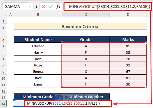
Here, in the VLOOKUP function, we inserted Cell range B14 as lookup_value, Cell range C5:D11 as table_array, 2 as col_index_num, and FALSE as range_lookup which represents an Exact match. Then, we used this value in the MIN function to get the Minimum Number.
- After that, press ENTER.
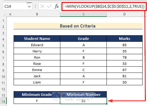
- Now, in this case, you will get the value that comes first in the range.

- Otherwise, insert the following formula in Cell C14.
=MIN(VLOOKUP($B$14,$C$5:$D$11,2,TRUE))
Here, in the VLOOKUP function, we inserted Cell range B14 as lookup_value, Cell range C5:D11 as table_array, 2 as col_index_num, and FALSE as range_lookup which represents an Exact match. Then, we used this value in the MIN function to get the Minimum Number.
- Finally, press ENTER.
Using Combined Functions to VLOOKUP & Return Multiple Matching Values in Excel
In the last method, we will show you how to VLOOKUP to return min value from multiple hits using the INDEX, SMALL, IF, ROW, MIN, and COLUMNS functions in Excel. You can use this method if you know under which criteria you want to find out the minimum value.

Follow the steps given below to do it on your own.
Steps:
- Firstly, select Cell C14.
- After that, insert the following formula.
=INDEX($C$5:$C$11,SMALL(IF($B$14=$D$5:$D$11, ROW($D$5:$D$11)-MIN(ROW($D$5:$D$11))+1, ""), COLUMNS($A$1:A1)))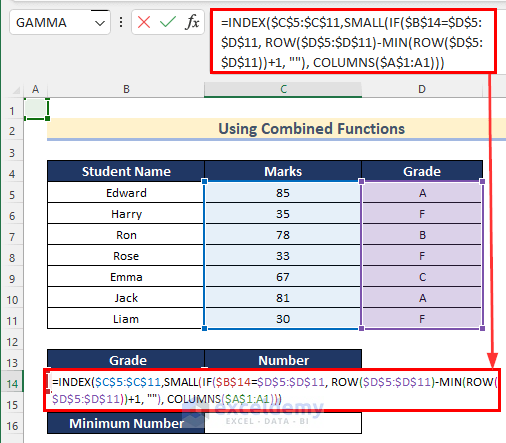
Formula Breakdown
- ROW($D$5:$D$11)—–> The ROW function returns the row number.
- Output: {“A”;”F”;”B”;”F”;”C”;”A”;”F”}
- COLUMNS($A$1:A1)—–> The COLUMNS function returns the column number.
- Output: {1}
- MIN(ROW($D$5:$D$11))—–> The MIN function returns the minimum value in a given range.
- MIN({5;6;7;8;9;10;11})—–> turns into
- Output: {5}
- MIN({5;6;7;8;9;10;11})—–> turns into
- IF($B$14=$D$5:$D$11, ROW($D$5:$D$11)-MIN(ROW($D$5:$D$11))+1, “”)—–> The IF function returns a value if the logical test is True and returns another value if it is False.
- IF($B$14=$D$5:$D$11,{5;6;7;8;9;10;11}-5+1, “”)—–> turns into
- Output: {“”;2;””;4;””;””;7}
- IF($B$14=$D$5:$D$11,{5;6;7;8;9;10;11}-5+1, “”)—–> turns into
- SMALL(IF($B$14=$D$5:$D$11, ROW($D$5:$D$11)-MIN(ROW($D$5:$D$11))+1, “”), COLUMNS($A$1:A1))—–> The SMALL function returns nth lowest or smallest value of a given range.
- SMALL({“”;2;””;4;””;””;7},1)—–> turns into
- Output: {2}
- SMALL({“”;2;””;4;””;””;7},1)—–> turns into
- INDEX($C$5:$C$11,SMALL(IF($B$14=$D$5:$D$11, ROW($D$5:$D$11)-MIN(ROW($D$5:$D$11))+1, “”), COLUMNS($A$1:A1)))—–> The INDEX function returns a value from a given single range.
- INDEX($C$5:$C$11,2)—–> turns into
- Output: {35}
- INDEX($C$5:$C$11,2)—–> turns into
- Then, press ENTER and drag right the Fill Handle tool to AutoFill the other values under Grade F.

- Now, you will get all the values under Grade F.

- Next, select Cell C16.
- After that, insert the following formula.
=MIN(C14:E14)
Here, in the MIN function, we inserted Cell range C14:E14 as number_1 to find out the minimum value under F Grade.
- Finally, press ENTER.

Read More: How to Use VLOOKUP Function on Multiple Rows in Excel
Use of MATCH Function to Return Matching Values from Multiple Min in Excel
Furthermore, you will find a way to VLOOKUP to return min value or its adjunct Cell value using INDEX, MATCH, and MIN functions in Excel here.
Steps:
- Firstly, select Cell B14.
- Then, insert the following formula.
=INDEX(D5:D11,MATCH(MIN(C5:C11),C5:C11,0))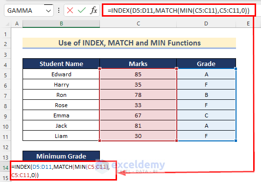
Formula Breakdown
- MIN(C5:C11)—–> The MIN function returns the minimum value in a given range.
- Output: {30}
- MATCH(MIN(C5:C11),C5:C11,0)—–> The MIN function returns the position of a lookup value.
-
- MATCH(30,C5:C11,0)—–> turns into
- Output: {7}
- MATCH(30,C5:C11,0)—–> turns into
- INDEX(D5:D11,MATCH(MIN(C5:C11),C5:C11,0))The INDEX function returns a value from a given single range.
- INDEX(D5:D11,7)—–> turns into
- Output: {F}
- INDEX(D5:D11,7)—–> turns into
- After that, press ENTER to get the value of Minimum Grade.

Practice Section
In this section, we are giving you the dataset to practice on your own and learn to use these methods.

Download Practice Workbook
Conclusion
So, in this article, you will find 4 ways for VLOOKUP to return min value from multiple hits. Use any of these ways to accomplish the result in this regard. Hope you find this article helpful and informative. Feel free to comment if something seems difficult to understand.
Related Articles
- Excel VLOOKUP to Return Multiple Values in One Cell Separated by Comma
- How to VLOOKUP Multiple Values in One Cell in Excel
- How to Use Excel VLOOKUP to Return Multiple Values Vertically
<< Go Back to VLOOKUP Multiple Values | Excel VLOOKUP Function | Excel Functions | Learn Excel
Get FREE Advanced Excel Exercises with Solutions!
