How to Use MIN Function in Excel (6 Relevant Examples)

In Microsoft Excel, the MIN function is used to extract the lowest or smallest value from a range of cells containing numerical data only. Here’s an overview of the common uses of this function.

Introduction to the MIN Function

Function Objective:

The MIN function extracts the lowest or smallest value from a range of cells or cell references.

Syntax:

=MIN(number1, [number2],…)

Arguments Explanation:

Argument	Required/Optional	Explanation
number1	Required	A range of cells, a cell reference, an array, or a numerical value.
[number2]	Optional	2nd numerical value or the range of cells.

Return Parameter:

The smallest number among a range of numerical values.

Using the MIN Function in Excel: 6 Suitable Examples

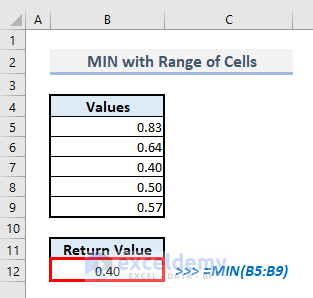
Example 1 – Using the MIN Function with a Range of Cells in Excel

Consider that the column B (B5:B9) has some numbers, and we’ll apply the MIN function to get the smallest value.

Steps:

Select the output cell B12 and insert:

=MIN(B5:B9)

Press Enter.

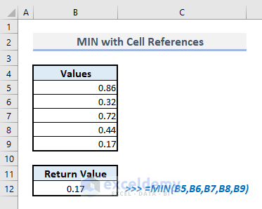
Example 2 – Using the MIN Function with Cell References or Direct Data Input

Steps:

In the output cell B12, use this formula:

=MIN(B5,B6,B7,B8,B9)

=MIN(0.86,0.32,0.72,0.44,0.17)

Hit Enter.

Example 3 – Applying the MIN Function with a Condition or Criteria in Excel

Although MINIF and MINIFS functions can fulfill the purposes of including conditions or criteria, you can also combine MIN and IF functions to find out the lowest data from a range of cells based on a certain condition. We’ll determine the lowest value from the range of cells in column B containing the decimal numbers greater than 0.50.

Steps:

In the output cell B15, use:

=MIN(IF(B5:B9>0.5,B5:B9,""))

Press Enter.

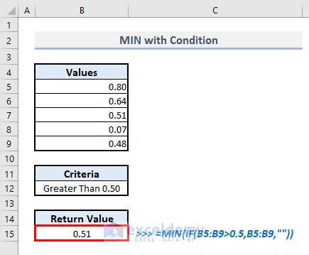
Here the IF function extracts the decimal values greater than 0.50 and then the MIN function shows the lowest value from the extracted data.

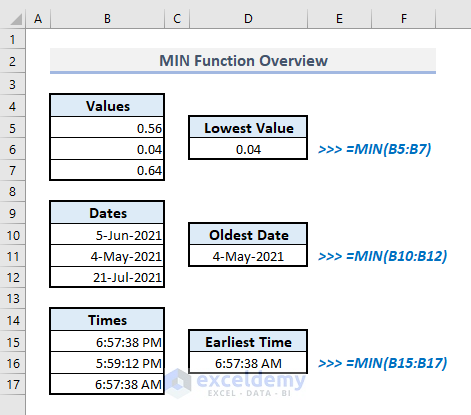
Example 4 – MIN Function to Find the Oldest Date from a Range of Cells in Excel

We have some date values in column B. We’ll pull out the oldest date among these values.

Steps:

Select the output cell B12 and use:

=MIN(B5:B9)

Press Enter and you’ll get the oldest date.

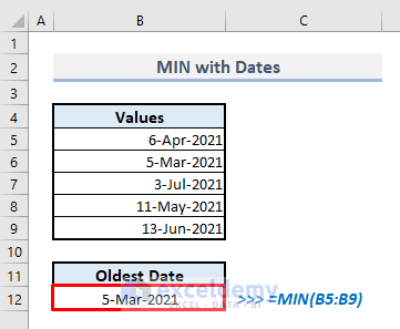
Dates are stored as serial numbers (starting from Jan 1, 1900), so each next day has a value 1 higher than the previous and older dates have lower values.

Read More: How to Find Minimum Value in Excel

Example 5 – MIN Function to Find the Earliest Time from a Range of Cells in Excel

In column B, we have a set of timestamps with H:MM:SS AM/PM format. We’ll apply the MIN function to find the earliest time.

Steps:

In cell B12, the related formula will be:

=MIN(B5:B9)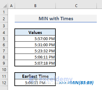

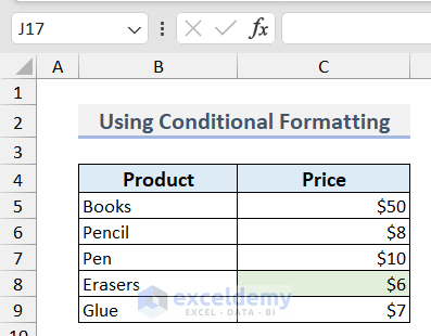
Example 5 – Highlight the Smallest Number Using Conditional Formatting

Select your desired cell range.
Go to the Home tab, click on Conditional Formatting, and select the New Rule option.

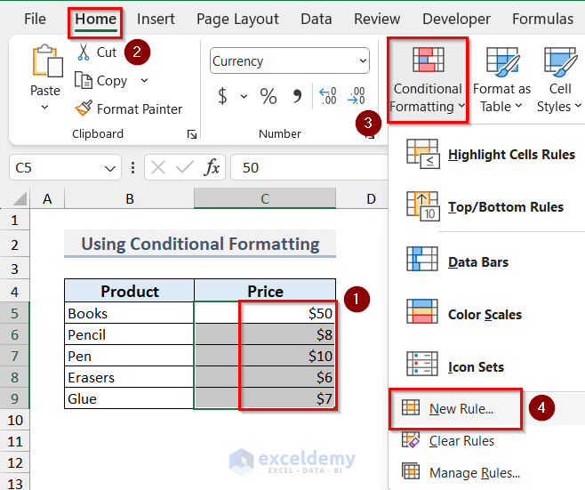
In the New Formatting Rule box, select the Format only top or bottom ranked values option.
Select Bottom and insert 1 in the box, then click on Format.

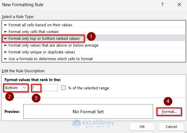
Select any format that you want and click on OK.
Click on OK again to apply the rule.
You will get the smallest number highlighted like the picture below.

How to Fix the MIN Function Not Working in Excel

The following errors may occur while using the MIN function in Excel.

#VALUE Error

Commonly shown for wrong arguments such as text values or the arguments going out of range.

#NUM! Error

This type of error is shown in Excel when the formula you have inserted is not possible to calculate.

#DIV/0! Error

This error is shown when a user tries to divide any number by zero. While using the MIN function, check if any data point shows #DIV/0! Error and solve it.

#NAME? Error

This error occurs for misspelled functions or wrong arguments. Check them to solve this issue. Also, this issue may occur if your numbers are text representations of numbers. Convert those text values to numbers first.

Things to Keep in Mind

The MIN function does not count blank cells. It’ll extract the lowest value from all other non-empty cells, or no value if the range is blank.
You can input up to 255 arguments in the MIN function.
The MIN function ignores boolean and text values as this function is assigned to extract data from numerical values only.
If you need to include a condition or criteria, use the MINIF or MINIFS functions.
If you want to input a logical value, then the MINA function should work instead.