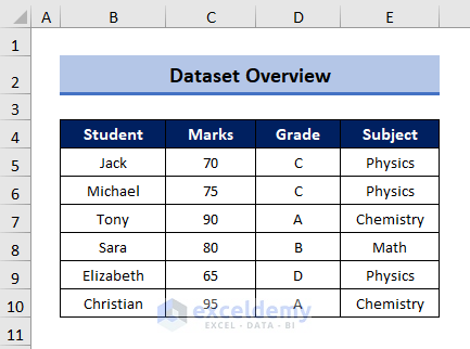
We will use the following data table to explain the methods to find minimum value with VLOOKUP in Excel.
Method 1 – Minimum Value with VLOOKUP Function
1.1 Find the Minimum Value
Steps:
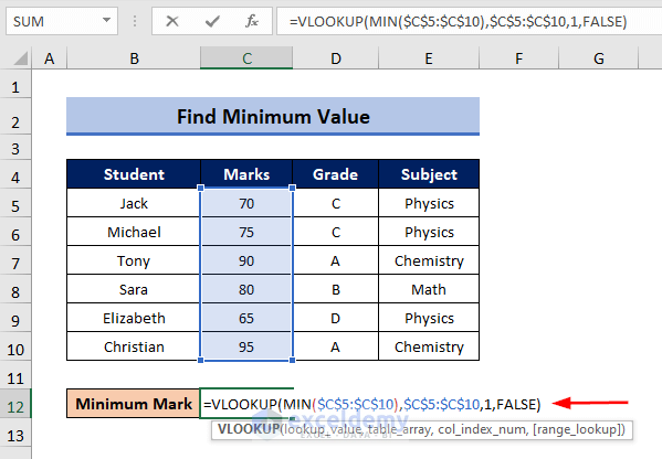
- Select the output Cell C12.
- Enter the following formula.
=VLOOKUP(MIN($C$5:$C$10),$C$5:$D$10,1,FALSE)
💡 Formula Breakdown
MIN($C$5:$C$10) will return the minimum value in the range $C$5:$C$10
$C$5:$D$10 is the table array, 1 is the column index number which is the Grade column, and FALSE is for Exact Match
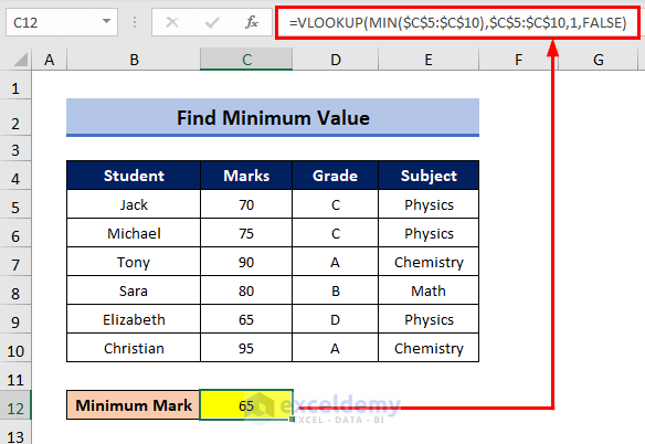
- Press ENTER.
You will find the Minimum Mark which is 65.
Read More: How to Find Minimum Value in Excel
1.2 Return the Adjacent Cell of the Minimum Value
Steps:
- Select the output cell C12.
- Enter this formula.
=VLOOKUP(MIN($C$5:$C$10),$C$5:$D$10,2,FALSE)
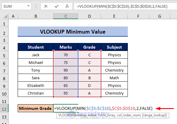
- Press ENTER.
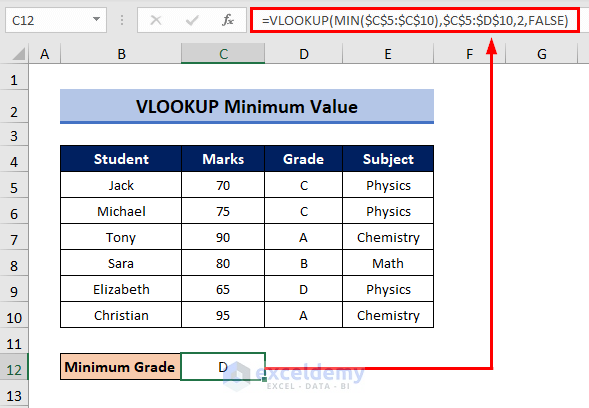
You will find the Minimum Grade which is Grade D.
1.3 Return Multiple Values with VLOOKUP
Steps:
- Select the output cell B13.
- Enter the following formula:
=VLOOKUP(MIN(C5:C10),$C$5:$E$10,{2,3},FALSE)
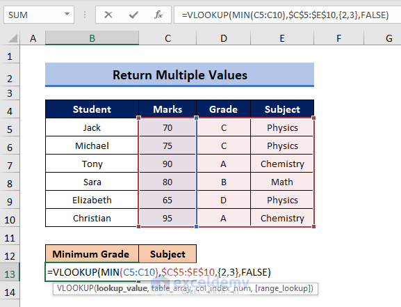
💡 Formula Breakdown
MIN(C5:C10) will return the minimum value in the range of C5:C10.
$C$5:$E$10 is the table array, {2,3} is the array of the column index number and FALSE is for Exact Match
- Press ENTER.
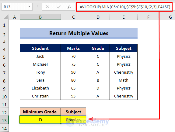
You will find the Minimum Grade which is D, and the corresponding subject Physics.
Method 2 – Using INDEX-MATCH Function
Steps:
- Select the Cell C12.
- Enter the following formula:
=INDEX(B5:B10,MATCH(MIN(C5:C10),C5:C10,0))
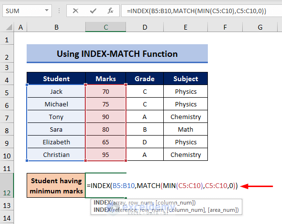
💡 Formula Breakdown
MIN(C5:C10) will return the minimum value in the range of C5:C10
C5:D10 is the lookup array, and 0 is for Exact Match.
B5:B10 is the range of student’s name that you want as a result.
- Press ENTER.
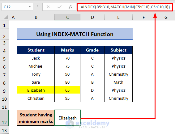
You will find the name of the student with the lowest mark.
Read More: How to Find Lowest 3 Values in Excel
Method 3 – Find the Nth Minimum Value with VLOOKUP
Steps:
- Select the output cell C12.
- Apply the following formula to find the 2nd minimum value.
=VLOOKUP(SMALL(C5:C10,2),C5:D10,2,FALSE)
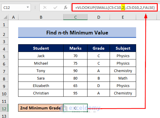
💡 Formula Breakedown
SMALL(C5:C10,2) will return the 2nd minimum value in the range C5:C10, where 2 is the kth value.
C5:D10 is the table array, 2 is the column index number which is the Grade column, and FALSE is for Exact Match.
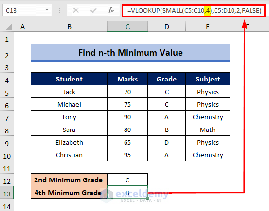
You will find the 2nd Minimum Grade which is Grade C.
- For getting the 4th minimum value, change the second argument of the SMALL function.
=VLOOKUP(SMALL(C5:C10,2),C5:D10,4,FALSE)
Read More: How to Find Lowest Value with Criteria in Excel
Method 4 – Using MINA with VLOOKUP Function
- Select the output cell C12.
- Enter the following formula:
=VLOOKUP(MINA(C5:C10),$C$5:$D$10,2,0)
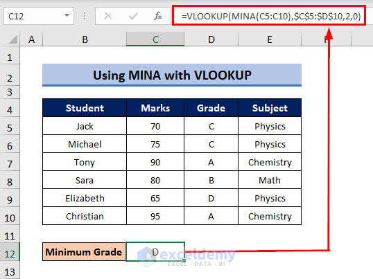
💡 Formula Breakdown
MINA(C5:C10) will return the minimum value in the range of C5:C10.
$C$5:$D$10 is the table array, 2 is the column index number which is the Grade column, and FALSE is for Exact Match.
You will find the Minimum Grade which is Grade D.
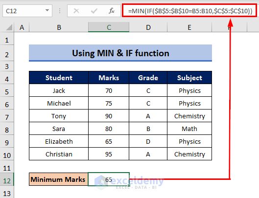
Method 5 – Using MIN and IF Functions
- Select the output cell C12.
- Enter the following formula:
=MIN(IF($B$5:$B$10=B5:B10,$C$5:$C$10))
💡 Formula Breakdown
B5:B10 is the range of Students and $C$5:$C$10 is the range of Marks.
$B$5:$B$10=B5:B10 is the logical test in the IF function and $C$5:$C$10 is the value when the logical test is TRUE.
You will find the Minimum Marks which is 65.
Read More: How to Use Combined MIN and IF Function in Excel
Method 6 – Use VLOOKUP to Find the Minimum Value in a Row
In the following table, there are 3 rows for marks of 3 subjects. To know the minimum mark for any of the subjects you have to find the minimum value row-wise. You can use the MIN function and the VLOOKUP function for this purpose.
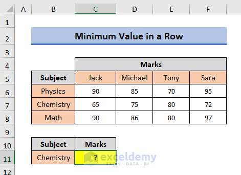
- Select the output cell C11.
- Apply the following formula:
=MIN(VLOOKUP(B11,$B$6:$F$8,{2,3,4,5},FALSE))
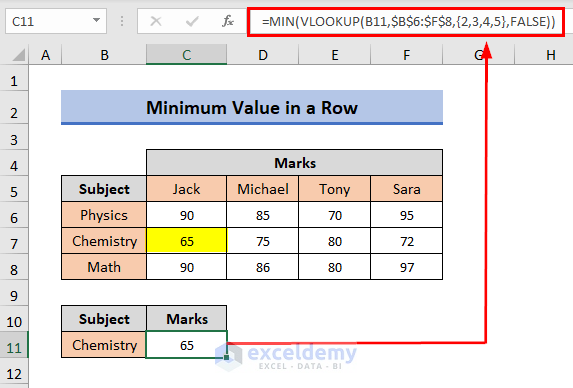
B11 is the lookup value, $B$6:$F$8 is the table array, {2,3,4,5} is the array of the column index number.
You will find the minimum mark which is 65 for Chemistry.
Read More: How to Find Minimum Value That Is Greater Than 0 in Excel
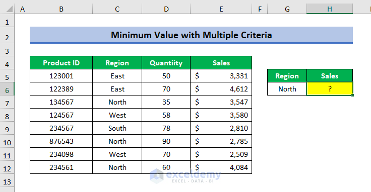
How to Find the Minimum Value with Multiple Criteria in Excel
We want to find the minimum sales for the North region, specifically for orders with a quantity greater than 60 in the sample dataset below.
Steps:
- Select the output Cell G6.
- Enter the following formula:
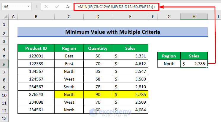
=MIN(IF(C5:C12=F6,IF(D5:D12>60,E5:E12)))
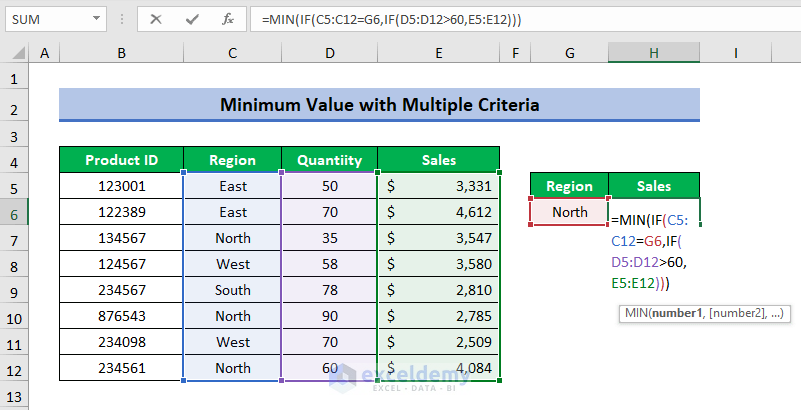
💡 Formula Breakdown
C5:C12 is the range of Region, D5:D12 is the range of Quantity and E5:E12 is the range of Sales.
C5:C12=F6 is the first logical test in the IF function and IF(D5:D12>60, E5:E12) is the value when the logical test is TRUE.
- Press ENTER and you will find the Minimum Sales which is $2,785.00.
Read More: How to Find Minimum Value Based on Multiple Criteria in Excel
Download the Practice Workbook
Related Articles
- How to Use MIN Function to Exclude Zero in Excel
- Excel MIN Function Returns 0
- Difference Between MAX and MIN Function in Excel
<< Go Back to Excel MIN Function | Excel Functions | Learn Excel
Get FREE Advanced Excel Exercises with Solutions!
