How to Find Lowest 3 Values in Excel: 5 Easy Ways

Method 1 – Using SMALL Function

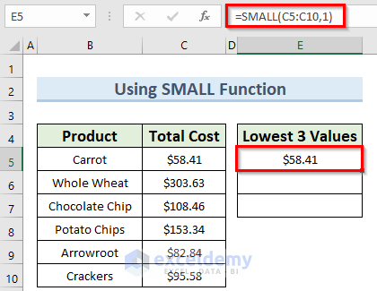
Step 1: Click on any cell E5. Insert the formula:

Step 2:  Press ENTER. The First lowest value will appear.

Repeat Steps 1-2 for cells E6 and E7 putting the k’s values 2 and 3 respectively. Get a picture similar to the picture below.

Repeating the steps we get the lowest 3 values $58.41, $82.84, and $95.58 in ascending order.

Method 2 – Utilizing SMALL Function Auto Rank

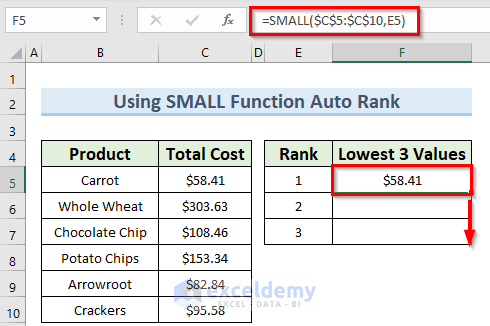
Step 1: To begin with, insert 1, 2, and 3 in any cell (E5, E6, E7) in a column.

Step 2: In the adjacent cell (F5), type:

Don’t forget to lock the range; you will end up with miscalculated data.

Step 3: Press ENTER. The First lowest value will appear.

Step 4: Drag the Fill Handle up to the last cell (F7), all 3 lowest values will appear.

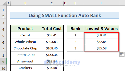
You can see that we have the same lowest 3 values as we have with Method 1 but with less effort.

Method 3 – Combining SMALL and ROW Functions

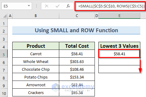
Step 1: Click on a cell (E5). Paste the formula:

Step 2: Hit ENTER. The utmost lowest value will appear.

Step 3: Drag the Fill Handle, and the rest of the values will show up.

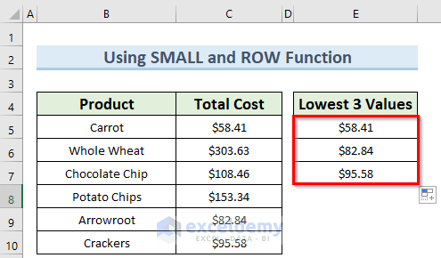
Find not only 3 lowest values but also n numbers of lowest values. As you can also see the values we get are similar to prior results.

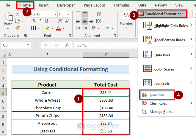
Method 4 – Implementing Conditional Formatting

Step 1: Select cells C5 to C10 and then go to Home Tab >> Conditional Formatting (in Style Section). Select New Rule.

Step 2: A new Formatting Rule window will pop up. Select “Use a formula to determine what cell to format” in the Select a rule box.

Step 3: Insert this formula in Edit the Rule Description box.

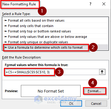
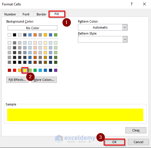
Step 4: Click on Format below the Edit the Rule Description box & Choose Fill Colour (Yellow).

Step 5: Click OK.

The consequences of these steps result in an image similar to the image below

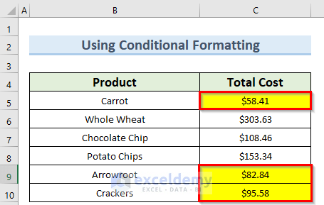
We can see Conditional Formatting colors with the 3 lowest values.

Method 5 – Applying AGGREGATE Function with SMALL Function

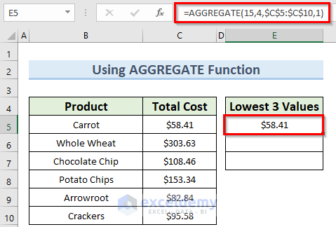
Step 1: Insert the formula in any cell (F5):

Step 2: Click OK. The outcome depicts the following image

Step 3: Repeat Steps 1 and 2, replacing the position number(k) with 2 and 3. Get something like the image below

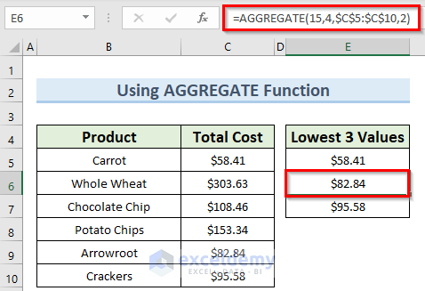
We can see that similar results are popping up with every method.

Download Practice Workbook

You can download the practice workbook from here.

Related Articles

• How to Use MIN Function to Exclude Zero in Excel
• Excel MIN Function Returns 0
• How to Find Minimum Value That Is Greater Than 0 in Excel
• Difference Between MAX and MIN Function in Excel

<< Go Back to Excel MIN Function | Excel Functions | Learn Excel