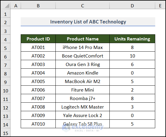
To find the minimum value and exclude zeros in a dataset or an array, you can use the MIN function.
This dataset includes Product ID, Product Name, and Units Remaining.
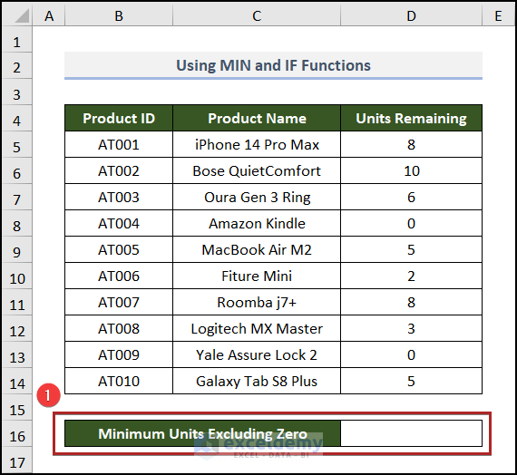
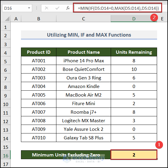
Method 1 – Using the MIN and IF Functions
Steps:
- Create an output field in the B16:D16 range.
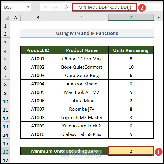
- Select D16 and enter the following formula.
=MIN(IF(D5:D14<>0,D5:D14))- IF(D5:D14<>0,D5:D14) → the IF function checks whether a condition is met, and returns one value if TRUE, and another one if FALSE. Here, the logical_test is D5:D14<>0 and the value_if_true argument is D5:D14. If the value of each cell in the D5:D14 range doesn’t equal 0, the function will return the value. Otherwise, it will return FALSE.
- Output → {8, 10, 6, FALSE, 5, 2, 8, 3, FALSE, 5}
- MIN(IF(D5:D14<>0,D5:D14)) becomes MIN(8, 10, 6, FALSE, 5, 2, 8, 3, FALSE, 5).
- MIN(8, 10, 6, FALSE, 5, 2, 8, 3, FALSE, 5) → the MIN function extracts the lowest or smallest value from a range of cells or cell references.
- Output → 2
- Press ENTER. If you are using older Excel versions press CTRL+SHIFT+ENTER.
Read More: How to Use Combined MIN and IF Function in Excel
Method 2 – Utilizing the MIN, IF, and MAX Functions
Steps:
- Go to D16 and insert the formula below.
=MIN(IF(D5:D14=0,MAX(D5:D14),D5:D14))Formula Breakdown
- MAX(D5:D14) → the MAX function returns the largest value in a given list of arguments.
- Output → 10
- IF(D5:D14=0,MAX(D5:D14),D5:D14) becomes IF(D5:D14=0,10,D5:D14).
- IF(D5:D14=0,10,D5:D14) → the IF function returns 10, when a cell value is equal to 0. Otherwise, it returns the same value.
- Output → {8, 10, 6, 10, 5, 2, 8, 3, 10, 5}
- MIN(IF(D5:D14=0,MAX(D5:D14),D5:D14)) becomes MIN(8, 10, 6, 10, 5, 2, 8, 3, 10, 5).
- MIN(8, 10, 6, 10, 5, 2, 8, 3, 10, 5) → returns the smallest among all numbers.
- Output → 2
- Press ENTER. If you are using older Excel versions press CTRL+SHIFT+ENTER.
Read More: How to Find Minimum Value in Excel
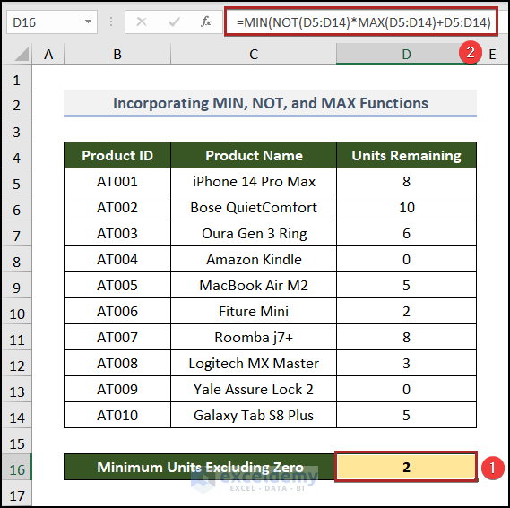
Method 3 – Incorporating the MIN, NOT, and MAX Functions
Steps:
- Select D16 and enter the formula below.
=MIN(NOT(D5:D14)*MAX(D5:D14)+D5:D14)Formula Breakdown
- MAX(D5:D14) → the MAX function returns the largest value in a given list of arguments.
- Output → 10
- NOT(D5:D14) → the NOT function reverses (opposite of) a Boolean or logical value. If you enter TRUE, the function returns FALSE, and vice versa.
- Output → {FALSE, FALSE, FALSE, TRUE, FALSE, FALSE, FALSE, FALSE, TRUE, FALSE}
- NOT(D5:D14)*MAX(D5:D14) becomes {FALSE, FALSE, FALSE, TRUE, FALSE, FALSE, FALSE, FALSE, TRUE, FALSE}*10
- Output → {0, 0, 0, 10, 0, 0, 0, 0, 10, 0}
- NOT(D5:D14)*MAX(D5:D14)+D5:D14 becomes {0, 0, 0, 10, 0, 0, 0, 0, 10, 0}+{8, 10, 6, 0, 5, 2, 8, 3, 0, 5}.
- Output → {8, 10, 6, 10, 5, 2, 8, 3, 10, 5}
- MIN(NOT(D5:D14)*MAX(D5:D14)+D5:D14) becomes MIN(8, 10, 6, 10, 5, 2, 8, 3, 10, 5).
- Output → 2
- Press ENTER. If you are using older Excel versions press CTRL+SHIFT+ENTER.
Read More: Difference Between MAX and MIN Function in Excel
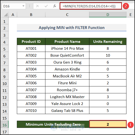
Method 4 – Applying the MIN and the FILTER Functions
Steps:
- Go to D16 and enter the formula below.
=MIN(FILTER(D5:D14,D5:D14<>0))The FILTER function filters particular cells or values. Here, the cell can’t be equal to zero. The rest of the formula is similar to the one in Method 1.
- Press ENTER. If you are using older Excel versions press CTRL+SHIFT+ENTER.
Read More: How to Find Lowest Value with Criteria in Excel
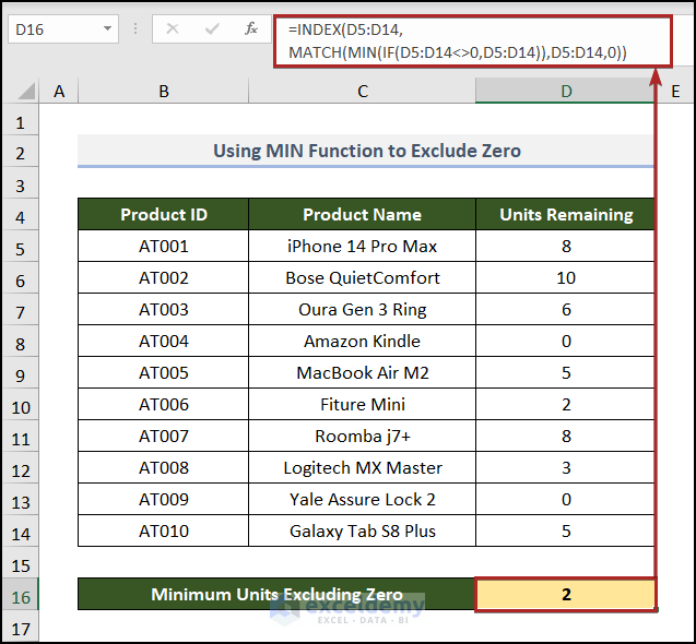
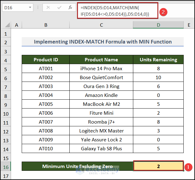
Method 5 – Implementing the INDEX-MATCH Formula and the MIN Function
Steps:
- Go to D16 and enter the following formula.
=INDEX(D5:D14,MATCH(MIN(IF(D5:D14<>0,D5:D14)),D5:D14,0))Formula Breakdown
- MIN(IF(D5:D14<>0,D5:D14)) → similar to Method 1.
- Output → 2
- MATCH(MIN(IF(D5:D14<>0,D5:D14)),D5:D14,0)) becomes MATCH(2,D5:D14,0)).
- MATCH(2,D5:D14,0)) → the MATCH function returns the lookup_value’s relative position. 2 is the lookup_value, D5:D14 is the lookup_array, and 0 for an exact match_type.
- Output → 6
- INDEX(D5:D14,MATCH(MIN(IF(D5:D14<>0,D5:D14)),D5:D14,0)) becomes INDEX(D5:D14,6).
- INDEX(D5:D14,6) → the INDEX function returns a value or reference of the cell at the intersection of a particular row and column in a given range.
- Output → 2
- Press ENTER. If you are using older Excel versions press CTRL+SHIFT+ENTER.
Read More: How to Find Minimum Value Based on Multiple Criteria in Excel
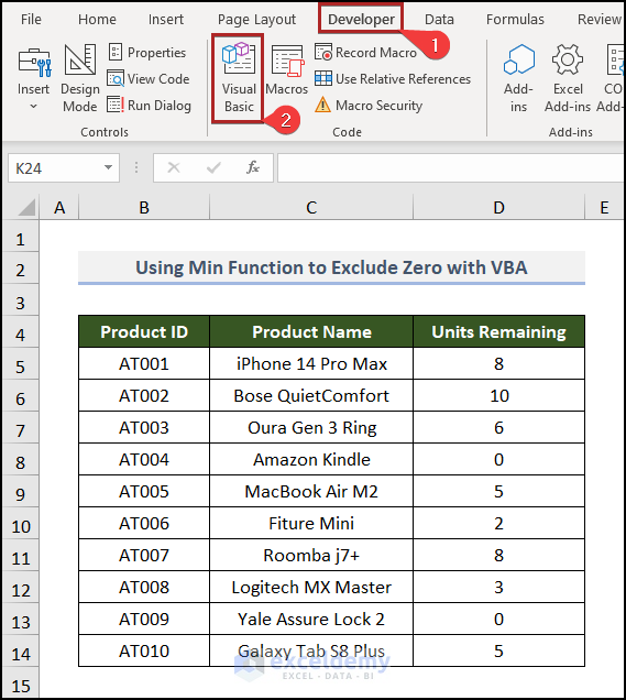
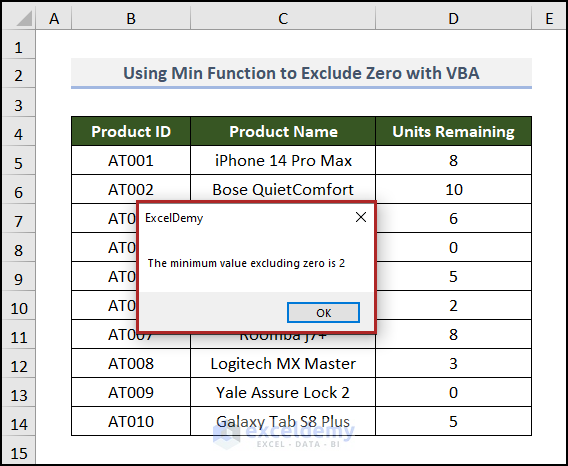
How to Use the Min Function to Exclude Zero Using VBA in Excel
Steps:
- Go to the Developer tab. In Code click Visual Basic.
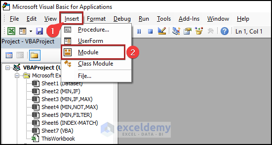
The Microsoft Visual Basic for Applications window opens.
- Go to the Insert tab.
- Select Module.
- Enter the following code in Module1.
Sub min_Exclude_zero()
MsgBox "The minimum value excluding zero is " & [min(if(D:D<>0,D:D))], vbOKOnly, "ExcelDemy"
End Sub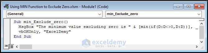
- Save the file as an Excel Macro-Enabled Workbook.
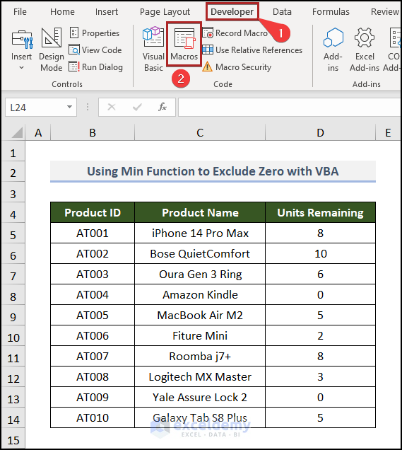
- Go back to the VBA worksheet.
- Go to the Developer tab.
- Click on Macros in the Code group.
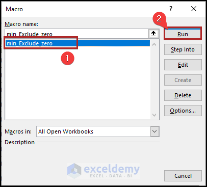
In the Macro dialog box:
- Select the only available macro.
- Click Run.
This is the output.
Read More: How to Find Minimum Value That Is Greater Than 0 in Excel
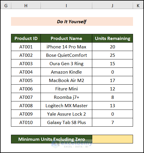
Practice Section
Practice here.
Download Practice Workbook
Download the Excel workbook to practice.
Related Articles
- How to Find Lowest 3 Values in Excel
- How to Find Minimum Value with VLOOKUP in Excel
- Excel MIN Function Returns 0
<< Go Back to Excel MIN Function | Excel Functions | Learn Excel
Get FREE Advanced Excel Exercises with Solutions!

You forget to mention that the MIN & IF options are array formulas, which have to be ended by CTRL+SHIFT+ENTER
Hello JJ,
Thank you for pointing that out! You’re right—the MIN & IF options are traditional array formulas that typically require CTRL+SHIFT+ENTER to work correctly. However, we used Excel 365, which supports dynamic arrays, so the formulas automatically spill without needing the key combination. We appreciate your feedback and will consider adding this clarification to help users of older Excel versions.
Regards
ExcelDemy