This is an overview:
The Excel NOT Function
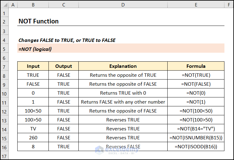
The NOT function reverses (opposite of) a Boolean or logical value. If you enter TRUE, the function returns FALSE, and vice versa.
Function Objective:
return a logically opposite value.
Syntax:
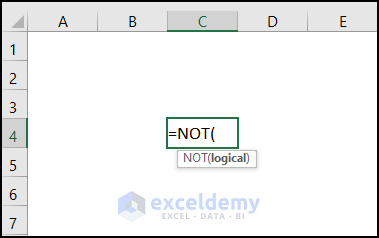
=NOT(logical)Argument Explanation:
| Argument | Required/Optional | Explanation |
|---|---|---|
| Logical | Required | A logical value that can be evaluated either TRUE or FALSE |
Return Parameter:
Reversed logical value: FALSE to TRUE, or TRUE to FALSE.
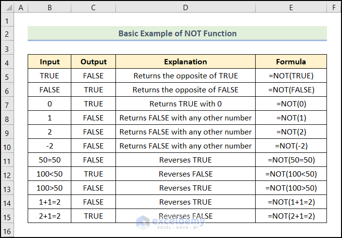
Example 1 – Basic Example of NOT Function in Excel
In the dataset below, B5 cell contains TRUE. The NOT function returns the opposite, FALSE. 0 is considered FALSE in Excel, so the NOT function returns TRUE with 0. For any other number, the output will be FALSE.
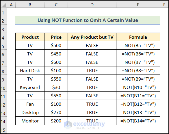
Example 2 – Excluding a specific Value Using the NOT Function
- Use the formula below:
=NOT(B5="TV")
B5 displays TV.
The function returns FALSE for TV and TRUE for all other products.
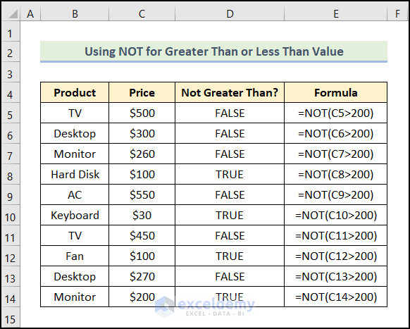
Example 3 – Using the NOT Function to Obtain a Greater Than or Less Than Value
To filter the products whose prices are less than $200, use:
=NOT(C5>200)
In C5, the Price of the TV is $500.
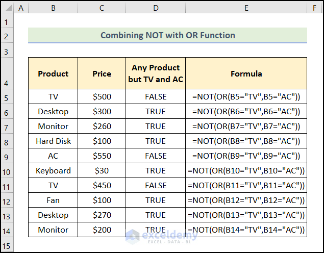
Example 4 – Checking If One or More Criteria Are Met
- Use the following formula:
=NOT(OR(B5="TV",B5="AC"))
B5 refers to TV.
Formula Breakdown:
- OR(B5=”TV”,B5=”AC”) → checks whether the arguments are TRUE, and returns TRUE or FALSE. It returns FALSE if all arguments are FALSE. Here, the functions check if the text in B5 is TV or AC: if one of the conditions is met, the function returns TRUE.
- Output → TRUE
- NOT(OR(B5=”TV”,B5=”AC”)) → becomes
- NOT(TRUE) → changes FALSE to TRUE, or TRUE to FALSE. Here, the function returns FALSE.
- Output → FALSE
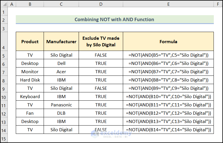
Example 5 – Ensuring Both Criteria Are Met in Excel
To exclude the Product TV made by Silo Digital:
=NOT(AND(B5="TV",C5="Silo Digital"))
B5 and C5 contain the Product TV and the Manufacturer Silo Digital.
Formula Breakdown:
- AND(B5=”TV”,C5=”Silo Digital”) → checks whether all the arguments are TRUE, and returns TRUE if all the arguments are TRUE. Here, B5=”TV” is the logical1 argument, and C5=”Silo Digital” is the logical2 argument. Since both conditions are met, the AND function returns the output TRUE.
- Output → TRUE
- NOT(AND(B5=”TV”,C5=”Silo Digital”)) → becomes
- NOT(TRUE) → the function returns the opposite of TRUE: FALSE.
- Output → FALSE
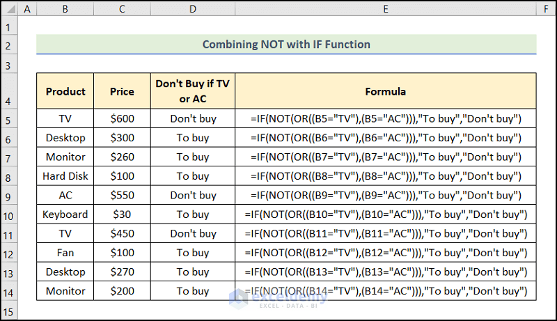
Example 6 – Constructing Logical Statements
- To avoid buying a TV or AC (the criteria), use the function:
=IF(NOT(OR((B5="TV"),(B5="AC"))),"To buy","Don't buy")
B5 refers to TV.
Formula Breakdown:
- OR((B5=”TV”),(B5=”AC”)) → checks whether the arguments are TRUE and returns TRUE or FALSE. It returns FALSE only if all arguments are FALSE. Here, the functions check if the text in B5 is TV or AC. If one of the conditions is met, the function returns TRUE.
- Output → TRUE
- NOT(OR(B5=”TV”,B5=”AC”)) → becomes
- NOT(TRUE) → changes FALSE to TRUE, or TRUE to FALSE. Here, the function returns the opposite of TRUE:FALSE.
- Output → FALSE
- IF(NOT(OR((B5=”TV”),(B5=”AC”))),”To buy”,”Don’t buy”) → becomes
- IF(FALSE,”To buy”,”Don’t buy”) → checks whether a condition is met and returns one value if TRUE and another value if FALSE. Here, FALSE is the logical_test argument because of which the IF function returns “Don’t buy” (the value_if_false argument). Otherwise, it returns “To buy” (the value_if_true argument).
- Output → “Don’t buy”
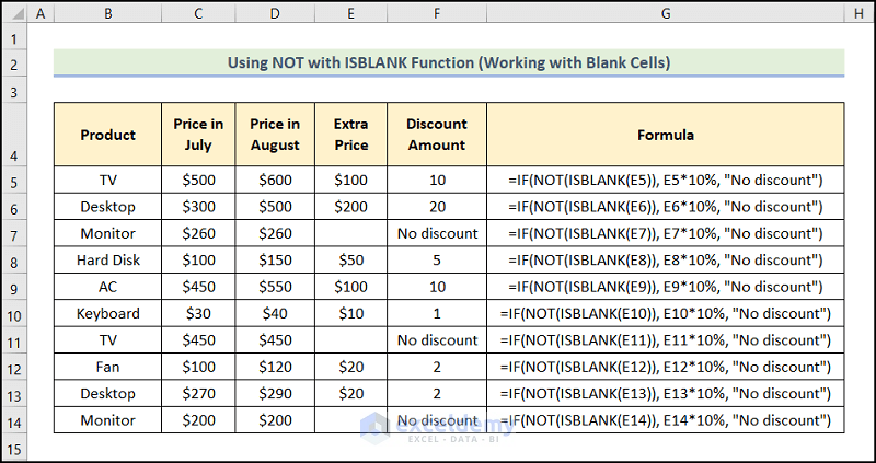
Example 7 – Checking for Blank Cells in Excel
- Use the formula:
=IF(NOT(ISBLANK(E5)), E5*10%, "No discount")
E5 indicates Extra Price.
Formula Breakdown:
- ISBLANK(E5) → checks whether a reference is an empty cell, and returns TRUE or FALSE. Here, E5 is the value argument that refers to Extra Price. The ISBLANK function checks whether the Extra Price cell is blank. It returns TRUE if blank and FALSE if not blank.
- Output → FALSE
- NOT(ISBLANK(E5)) → becomes
- NOT(FALSE) →, the function changes FALSE to TRUE.
- Output → TRUE
- IF(NOT(ISBLANK(E5)), E5*10%, “No discount”) → becomes
- IF(TRUE,E5*10%, “No discount”) → TRUE is the logical_test argument because of which the IF function returns E5*10% (the value_if_true argument). Otherwise, it would return “No discount” (the value_if_false argument).
- 100 * 10% → 10
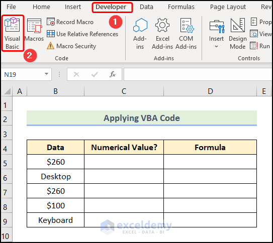
Example 8 – Applying a VBA Code
Steps:
- Go to the Developer tab >> click Visual Basic.
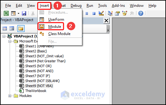
In the Visual Basic Editor:
- Go to the Insert tab >> select Module.
- Copy the code below.
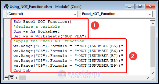
Sub Excel_NOT_Function()
'declare a variable
Dim ws As Worksheet
Set ws = Worksheets("NOT VBA")
'apply the Excel NOT function
ws.Range("C5").Formula = "=NOT(ISNUMBER(B5))"
ws.Range("C6").Formula = "=NOT(ISNUMBER(B6))"
ws.Range("C7").Formula = "=NOT(ISNUMBER(B7))"
ws.Range("C8").Formula = "=NOT(ISNUMBER(B8))"
ws.Range("C9").Formula = "=NOT(ISNUMBER(B9))"
End Sub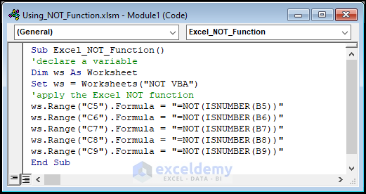
Code Breakdown:
- the sub-routine is named Excel_NOT_Function().
- defines the variable ws to store the Worksheet object and enter the worksheet name, here “NOT VBA”.
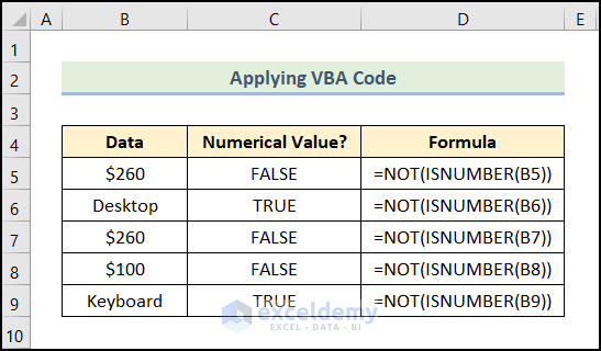
- the NOT and ISNUMBER functions check if the specified B5, B6, B7, B8, and B9 cells (input cells) contain numeric or text data.
- the Range object is used to return the result in C5, C6, C7, C8, and C9 (output cells).
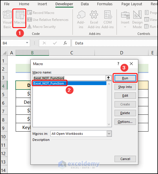
- Close the VBA window >> click Macros.
In the Macros dialog box:
- Select the copy_and_paste_data macro >> click Run.
This is the output.
Common Errors While Using the NOT Function
| Error | Occurrence |
|---|---|
| #VALUE! | the cell range is inserted as input |
Practice Section
Practice here.

Download Practice Workbook
<< Go Back to Excel Functions | Learn Excel
Get FREE Advanced Excel Exercises with Solutions!
