Method 1 – Application of NOT Boolean Operator
Step 1:
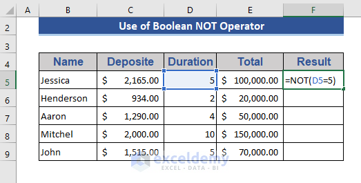
- Go to Cell F5.
- Write the below code:
=NOT(D5=5)
Step 2:
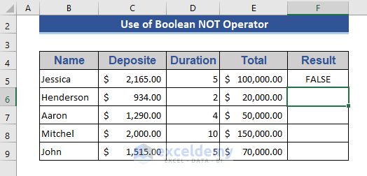
- Press Enter.
Step 3:
- Pull the Fill Handle towards the last cell.
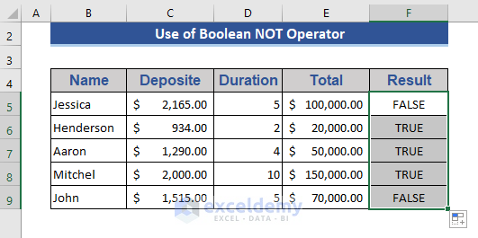
We applied the NOT function with a view to see which data of the cells of the Duration column is equal to 5 years. From the result, we can see that those cells that are equal to 5 are showing FALSE and the rest are showing TRUE.
Example 2:
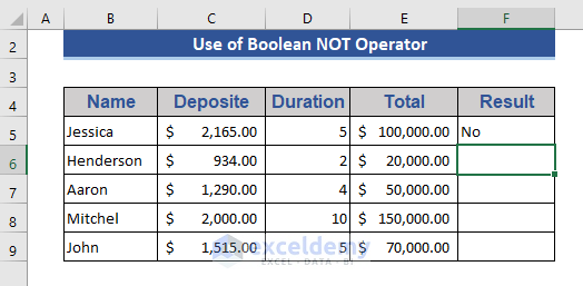
Insert the IF function with the NOT function.
Step 1:
- Write the following formula in Cell F5.
=IF(NOT(D5=5),"Yes","No")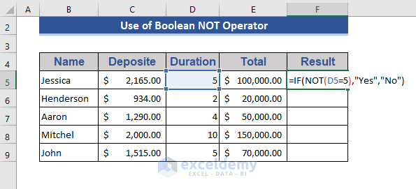
Step 2:
- Press Enter and see the return.
Step 3:
- Drag the Fill Handle icon towards the last cell.
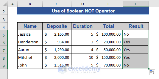
As the NOT function returns the reverse logical output, we also set a negative result for each cell.
One of the advantages of using the IF function is that we can set the return argument according to our desire.
Method 2 – Use of Boolean AND Operator in Excel
Step 1:
- Go to Cell F5 and put the formula below:
=AND(D5>5)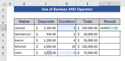
Step 2:
- Press Enter to get the return.
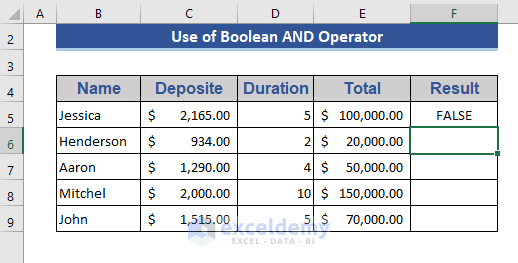
Step 3:
- Pull the Fill Handle icon towards the last cell.
See how simple to apply the AND operator.
Example 2:
In this example, we will apply multiple conditions in a single formula by applying the AND function each time. We will identify which rows contain a duration more than or equal to 5 years and the total loan is less than $100,000.
Step 1:
- Go to the Cell F5.
- Put the below formula which contains two conditions.
=AND(D5>=5,E5<=100000)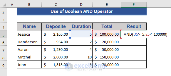
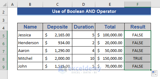
Step 2:
- See the return after applying the formula in the below image.
Apply multiple conditions with a single AND function in Excel.
Example 3:
Apply the nested AND function. Only AND function is used in the formula. Now, see what happens after applying this formula.
Step 1:
- Write the below formula on Cell F5.
=AND(AND(D5>2,D5<10),AND(E5>50000,E5<200000))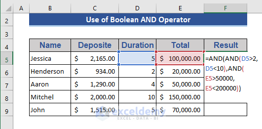
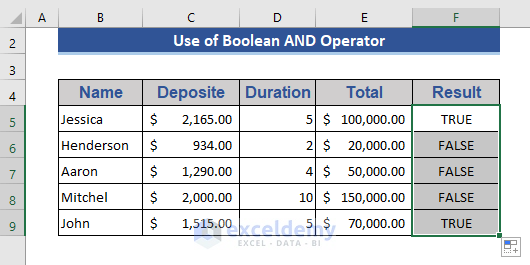
Step 2:
- Press Enter and apply for the rest of the cells also.

We planned the formula in the following way. Duration is greater than 2 years and less than 10 years. The total loan is greater than $50,000 and less than $200,000.
Example 4:
Insert the If a function with the AND operator. In this way, we can add manipulate the result as per our likings.
Step 1:
- Apply this formula on Cell F5.
=IF(AND(AND(D5>2,D5<10),AND(E5>50000,E5<200000)),"Success", "Failure")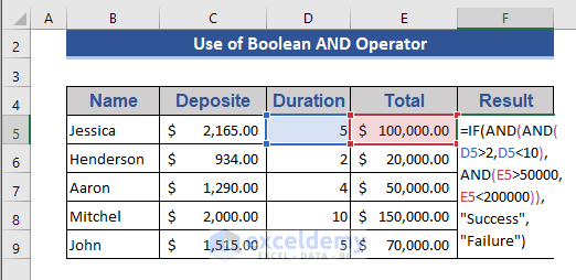
Step 2:
- Run the formula and see what happens.
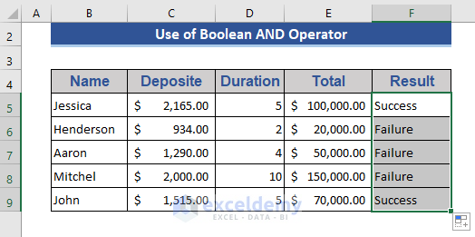
See that the return value is changed. “Success” and “Failure” are set instead of the default.
Example 5:
We can also apply the Cell range without individual cells along with the AND function.
We want to see if the deposit amount is greater than $1000.
Step 1:
- Apply the formula with range C5:C9 in Cell F5.
=AND(C5:C9>1000)
Step 2:
- Get the output after pressing Enter

We used a cell range instead of an individual cell number. This also performs smoothly.
Method 3 – Apply OR Operator in Excel
Example 1:
Find rows whose duration is greater than 5 years or the total loan is greater than $90,000. We applied two conditions in a single formula.
Step 1:
- Go to Cell F5.
- Write the below formula on that cell-
=OR(D5>5,E5>90000)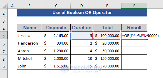
Step 2:
- Press Enter.
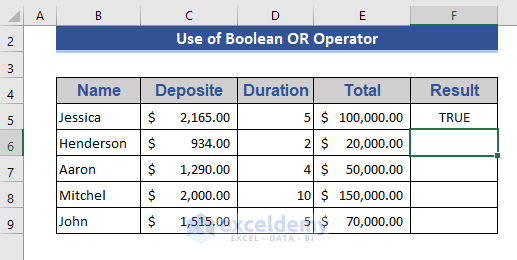
Step 3:
- Drag the Fill Handle icon to Cell F9.
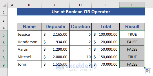
In the case of OR function, it provides TRUE as any of the conditions fulfilled.
Example 2:
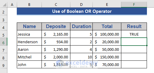
Apply cell range instead of an individual cell in this example. We want to know if the deposit money is greater than $2000.
Step 1:
- Insert the formula below to know if any of the deposits is greater than $2000.
=OR(C5:C9>2000)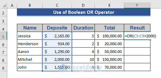
Step 2:
- Press Enter to get the result.
Example 3:
Apply a nested function. AND and IF function will also be inserted in the formula. We want to find which objects have a duration greater than 5 years or a total loan greater than or equal to $90,000 and deposit money is greater than $2000.
Step 1:
- Write the following formula on Cell F5.
=IF(OR(OR(D5>5,E5>=90000),AND(C5>2000)),"Yes","No")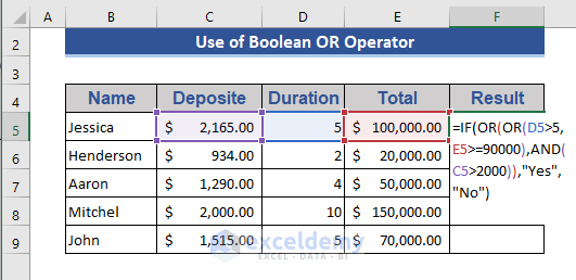
Step 2:
- Press Enter and get the result.
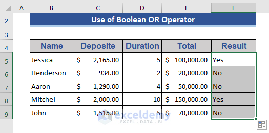
This is our nested output after applying the boolean operators.
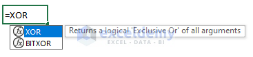
Method 4 – Function of XOR Operator in Excel
The XOR operator is commonly called “Exclusive OR.” It justifies in three ways. If all the arguments are true, then it returns FALSE. If any of the arguments is true, it returns TRUE. If all the arguments are false, it returns FALSE.
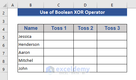
To explain this operator, we introduced a new data set. See the below data set.
First, each player plays 2 rounds. Head means winning of a player, and tail means loss. In the two rounds, if any player wins, i.e., gets head in both rounds, he does not need to play the 3rd round. If any player gets tails in both rounds, he will be disqualified from the game. And if the result is mixed, then he will get a chance to play 3rd round. This scenario can be explained easily by the XOR operator.
Step 1:
- After the 2 rounds, the result is updated in the data set.
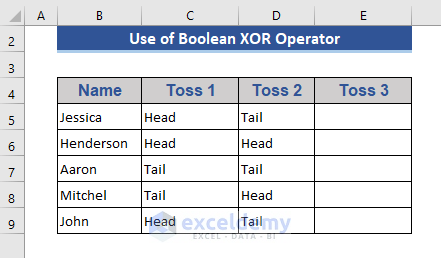
Apply the XOR function to identify who will play the 3rd round.
Step 2:
- Apply the formula on Cell F5.
=XOR(C5="Head",D5="Head")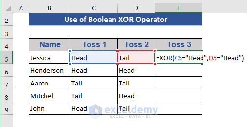
Step 3:
- Press Enter and drag won the Fill Handle
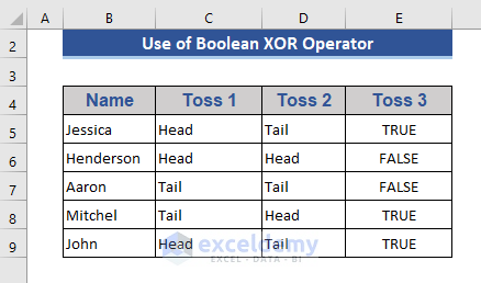
We get the result. As the result is showing in terms of TRUE and FALSE, it may be suitable all to understand easily.
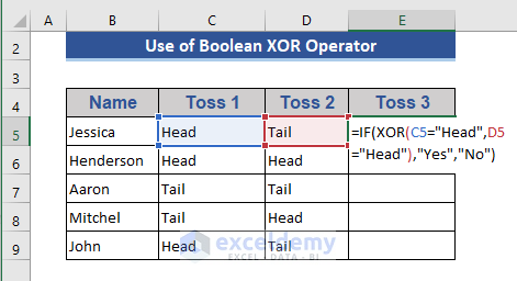
Insert the IF function to make it easier for all.
Step 4:
- After inserting the IF function, the formula will look like this.
=IF(XOR(C5="Head",D5="Head"),"Yes","No")
Step 5:
- Get a clear idea from the result below.
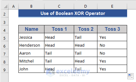
We can say now that 3 players will play the 3rd round and 2 players will not play.
Download Practice Workbook
Download this practice workbook to exercise while you are reading this article.
Related Articles
- How to Use Comparison Operators in Excel
- How to Perform Greater than and Less than in Excel
- How to Use Greater Than or Equal to Operator in Excel Formula
- How to Apply ‘If Greater Than’ Condition In Excel
- How Use Less Than Or Equal to Operator in Excel
- ‘Not Equal to’ Operator in Excel
- Reference Operator in Excel
- What is the Order of Operations in Excel
<< Go Back to Excel Operators | Excel Formulas | Learn Excel
Get FREE Advanced Excel Exercises with Solutions!
