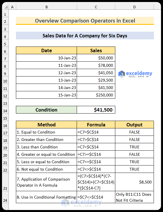
In this article, we will show you eight simple examples of how to use comparison operators in Excel. We will be using Microsoft 365 to do this; however, you can use any version of Microsoft Excel and follow this tutorial. The following image shows the overview of the methods for this article.
How to Use Comparison Operators in Excel: 8 Suitable Examples
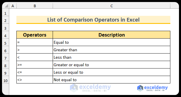
There will be 8 examples to use the comparison operators in Excel. In the first six exercises, we will show you the use of the operators in standalone scenarios. Then, in Example 7, you will see how to use the operators inside a formula. Lastly, we will use the operators inside the conditional formatting. Additionally, there are six comparison operators in Excel. The following image lists them all.
Example 1: Use of Equal To Operator
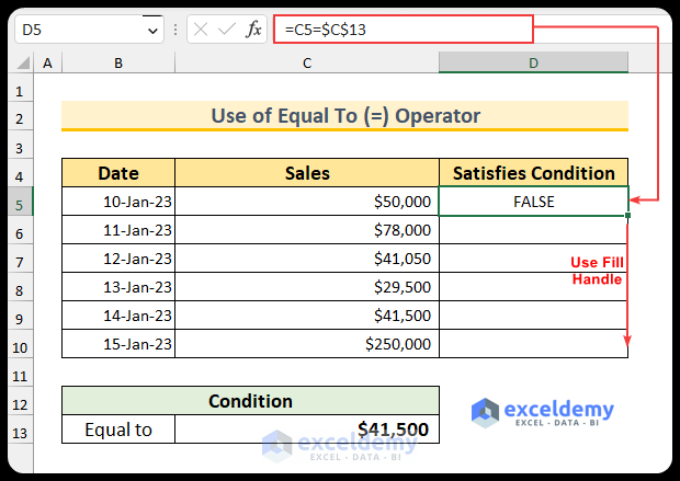
In the first example, we will see the use of the “Equal To (=)” operator from the comparison operators in Excel. We have a condition set, which is in cell C13. We will check if the values in the range C5:C10 are equal to that value or not.
Steps:
- Firstly, type the following formula in cell D5 and press Enter.
=C5=$C$13
- We can see that $50,000 is greater than the condition, so it has returned false.
- Secondly, use the Fill Handle to fill the formula into the rest of the cells. Notice, we have used the absolute cell reference for the condition, as it will always be the same for the formulas.
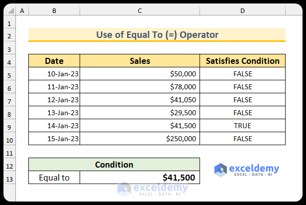
- Finally, after doing that, the dataset will look like this. Moreover, we can see that only the fifth sale value is equal to the condition.
Read More: How to Apply ‘If Greater Than’ Condition In Excel
Example 2: Application of Greater Than Operator
In the second example, we will see the use of the “Greater Than (>)” operator from the comparison operators. We have a condition set, which is in cell C13. We will check whether or not the values in the range C5:C10 are larger than the value.
Steps:
- Firstly, select the cell range D5:D10.
- Secondly, type the following formula.
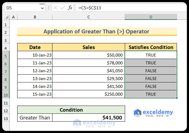
=C5>$C$13
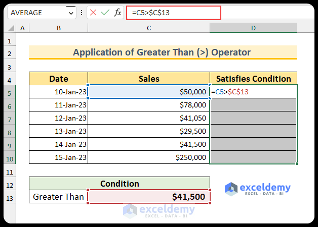
- Thirdly, press Ctrl+Enter.
- So, the formula will show us there are three values that satisfy our condition.
Example 3: Use of Less Than Operator in Excel
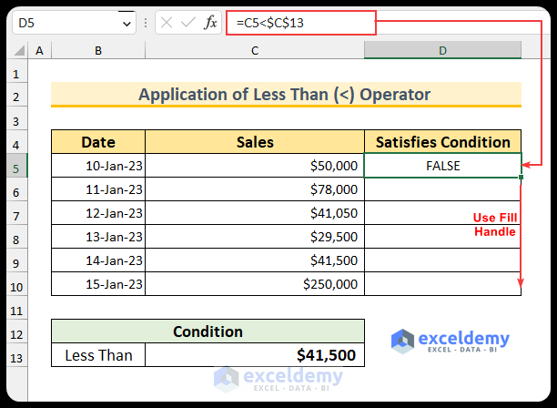
In the third example, we will see the use of the “Less Than (<)” operator from the comparison operators in Excel. We have a condition set, which is in cell C13. We will check if the values in the range C5:C10 are smaller than that value or not.
Steps:
- To begin with, type the following formula in cell D5 and press Enter.
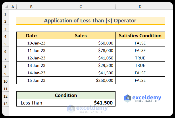
=C5<$C$13
- We can see that $50,000 is greater than the condition, so it has returned false.
- Secondly, use the Fill Handle to fill the formula into the rest of the cells.
- Finally, after doing so, we can see that only two values satisfy our condition.
Read More: How to Perform Greater than and Less than in Excel
Example 4: Use of Greater Or Equal To Operator
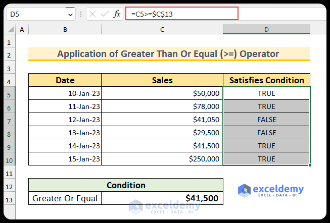
In the fourth example, we will see the use of the “Greater Than Or Equal To (>)” operator from the comparison operators. We have a condition set, which is in cell C13. We will check if the values in the range C5:C10 are larger than or equal to the value or not.
Steps:
- Firstly, select the cell range D5:D10.
- Secondly, type the following formula.
=C5>=$C$13
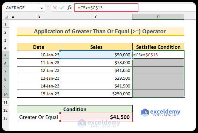
- Thirdly, press Ctrl+Enter.
- So, the formula will show us there are four values that satisfy our condition.
Read More: How to Use Greater Than or Equal to Operator in Excel Formula
Example 5: Utilization of Less Or Equal To Operator
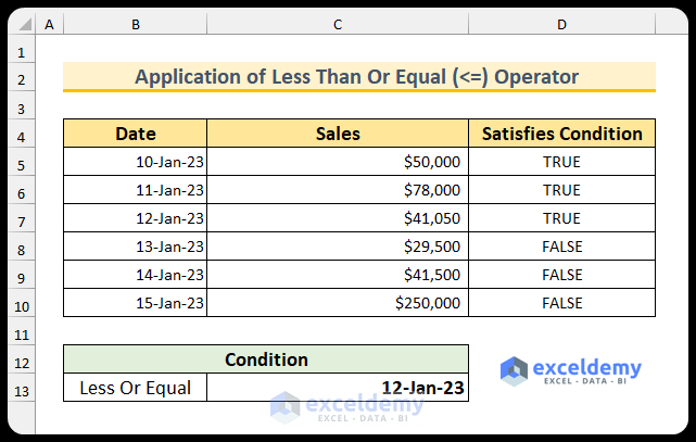
In the section, we will see the use of the “Less Than Or Equal To (<=)” operator from the comparison operators in Excel. Moreover, in this section, we will use the date values for demonstration. We have a condition set, which is in cell C13. We will check if the values in the range B5:B10 are smaller than or equal to that value or not.
Steps:
- To begin with, type the following formula in cell D5 and press Enter.
=B5<=$C$13
- We can see that “10-Jan-23” is smaller than the condition, so it has returned true.
- Secondly, use the Fill Handle to fill the formula into the rest of the cells.
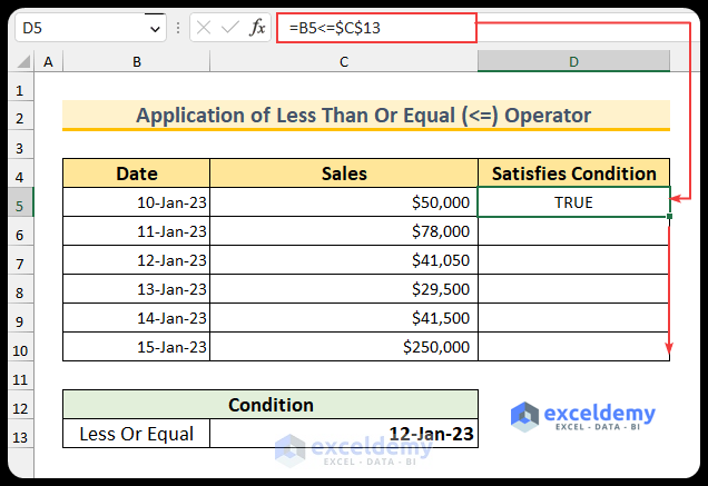
- Finally, after doing so, we can see that only three values satisfy our condition.
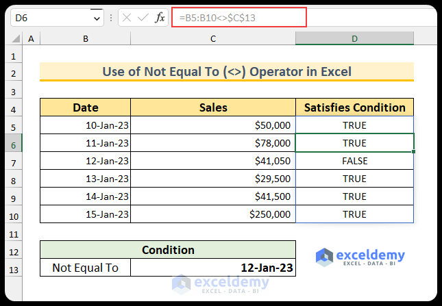
Example 6: Use of Not Equal To Operator in Excel
In the section, we will see the use of the “Not Equal To (<>)” operator in Excel. Again, in this section, we will use the date values for demonstration. We have a condition set, which is in cell C13. We will check if the values in the range B5:B10 are smaller than or equal to that value or not.
Steps:
- To begin with, type the following formula in cell D5.
=B5:B10<>$C$13
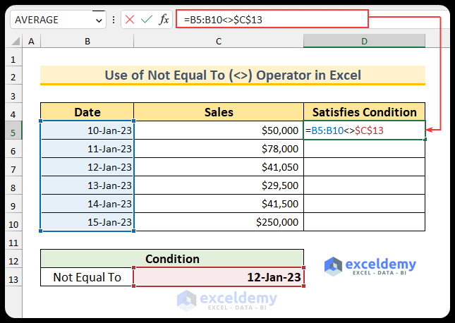
- Finally, press Enter. Then, we will see that all values except one satisfy our criteria.
Example 7: Use of Comparison Operators in Formula
We will show you the steps to use the comparison operators in a formula. For this example, we will calculate the difference between the sales values and the condition value. Moreover, the result will always be positive.
Steps:
- Firstly, type the following formula in cell D5.
=(C5>$C$13)*(C5-$C$13)+(C5<$C$13)*($C$13-C5)
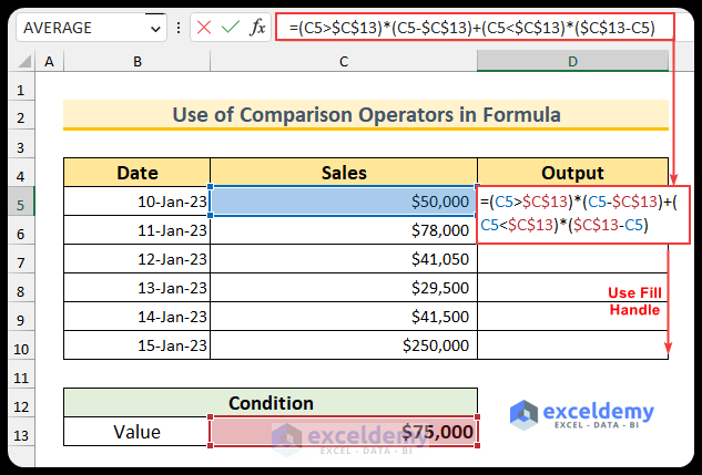
- Secondly, press Enter and use the fill the formula below.
- Lastly, the output will be similar to the snapshot below.
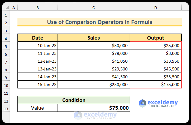
Formula Breakdown
- There are two parts in the formula. The first one is (C5>$C$13)*(C5-$C$13)
- When the cell value of C5 is greater than the cell value from C13, it returns true or 1.
- After that, it will multiply this 1 by the difference between these two values. For cell C5, the value is smaller than the condition. So, it will return false or 0. So the multiplication will also be 0.
- Similarly, the second part of this formula (C5<$C$13)*($C$13-C5) works.
- For cell C5, the value is smaller than the condition. So, it will return true or 1. So the multiplication will be ($75,000-$50,000)*1, or $25,000.
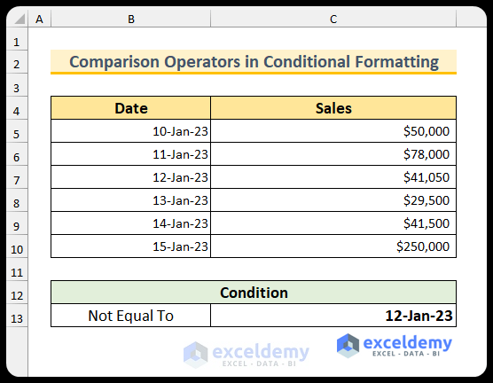
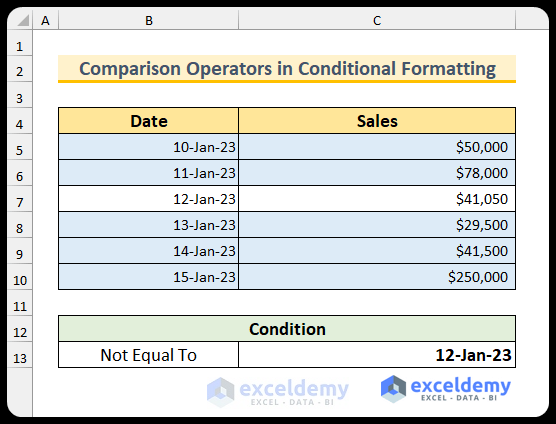
Example 8: Application of Comparison Operators in Conditional Formatting
We will show you how to apply the comparison operators in conditional formatting in Excel in this section. We have modified the dataset a little bit for this example.
Steps:
- To begin with, select the cell range B5:C10.
- Then, from the Home tab, select “New Rule…” from the Conditional Formatting.
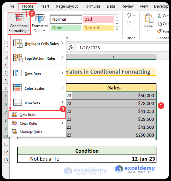
- So, a dialog box will pop up.
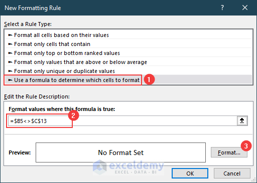
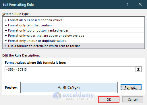
- Then, select “Use a formula to determine which cells to format” from the Select a Rule Type section.
- After that, type the following formula.
=$B5<>$C$13
- After that, press “Format…”.
- Then, from the Fill tab, select any color (we have selected the light blue color) and press OK.
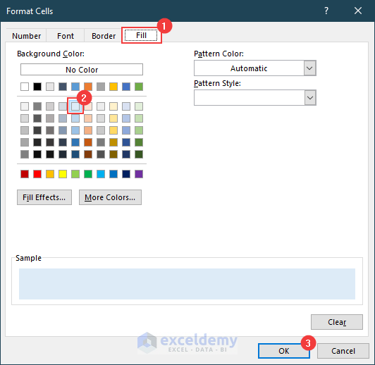
- Afterward, press OK again.
- Finally, we will highlight the cells which are not equal to the condition.
Download Practice Workbook
You can download the Excel file from the link below.
Conclusion
We have shown you 8 examples of comparison operators in Excel. Moreover, there is a practice section in the Excel file. You can use that to follow along with this article. Please comment below if you have any questions or concerns about these techniques. However, remember that our website implements comment moderation. Therefore, your comments may not be instantly visible. So, have a little bit of patience, and we will solve your query as soon as possible. Thanks for reading, keep excelling!
Related Articles
- Excel Boolean Operators: How to Use Them?
- How to Use Logical Operators in Excel
- Reference Operator in Excel
- What Is the Order of Operations in Excel
<< Go Back to Excel Operators | Excel Formulas | Learn Excel
Get FREE Advanced Excel Exercises with Solutions!
