Monte Carlo Simulation with the Microsoft Stack

 

Most analysts present uncertainty as a single number. A project will cost $2 million. Revenue will hit $5 million. These estimates feel precise, but they are almost certainly wrong. Monte Carlo simulation is a practical method for modeling uncertainty. Instead of assuming that one fixed value will happen, a Monte Carlo model runs many possible outcomes using random inputs. This helps answer questions such as: “What is the probability of losing money?”, “What is the expected profit range?”, or “How much risk is involved in this decision?”

In this tutorial, we will build a Monte Carlo simulation using the Microsoft Stack. We will use Excel to build the simulation engine, Power BI to visualize the probability distribution and scenario outcomes, and PowerPoint to present the results clearly to decision-makers.

Step 1: Setting Up the Model in Excel

Consider a project cost estimation example: estimating the total cost for a software development project with uncertain task costs and durations. Open a new Excel workbook. Create three sheets:

• Assumptions
• Model
• Simulations

1.1. Assumptions Sheet or Top of Model Sheet

Define uncertain variables with 3-point estimates (Minimum, Most Likely, Maximum) for triangular/PERT distributions, which are common in project risk analysis.

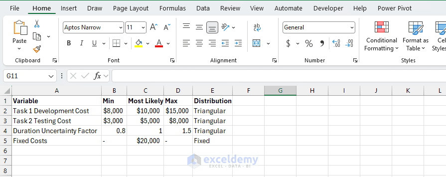
Why the triangular distribution? It is simple, widely used in project management (e.g. PERT), and requires only three intuitive estimates: pessimistic, most likely, and optimistic.

1.2. Model Sheet: Single Iteration Logic

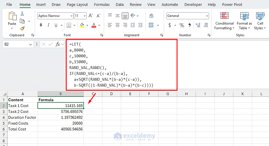
For triangular distribution sampling (approximate via NORMINV or a custom formula; for simplicity, many practitioners use a PERT-like beta approximation or a direct inverse), use the following practical formulas for a triangular random variable (Min=A, ML=C, Max=B). Place them in cells for one iteration.

• Task 1 Cost:

=LET(
a,8000,
c,10000,
b,15000,
RAND_VAL,RAND(),
IF(RAND_VAL<=(c-a)/(b-a),
  a+SQRT(RAND_VAL*(b-a)*(c-a)),
  b-SQRT((1-RAND_VAL)*(b-a)*(b-c))))

• Task 2 Cost:

=LET(
a,3000,
c,5000,
b,8000,
RAND_VAL,RAND(),
IF(RAND_VAL<=(c-a)/(b-a),
  a+SQRT(RAND_VAL*(b-a)*(c-a)),
  b-SQRT((1-RAND_VAL)*(b-a)*(b-c))))

• Duration Factor:

=LET(
a,0.8,
c,1,
b,1.5,
RAND_VAL,RAND(),
IF(RAND_VAL<=(c-a)/(b-a),
  a+SQRT(RAND_VAL*(b-a)*(c-a)),
  b-SQRT((1-RAND_VAL)*(b-a)*(b-c))))

• Total Project Cost:

=B5+(B2+B3)*B4

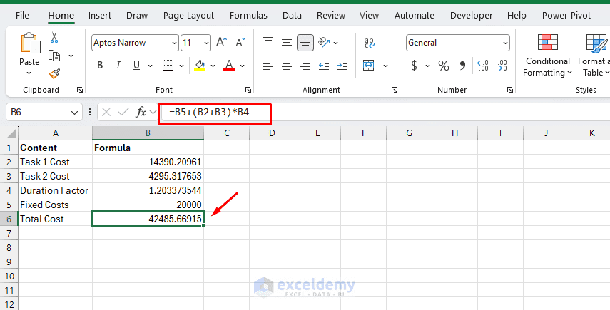
This sheet calculates one possible project outcome. The Total Cost cell is the output we will simulate thousands of times.

Step 2: Run Thousands of Simulations with Data Tables

This is the core "engine" — no coding required. Instead of a single "expected" number, we will generate 10,000 possible outcomes and analyze the full probability distribution of total project cost.

• In a new sheet named "Simulations":
  • A1: Simulation # (1 to 10,000)
  • B1: Total Cost
• Enter 1 in cell A2, and in cell A3 insert the following formula:

=A2+1

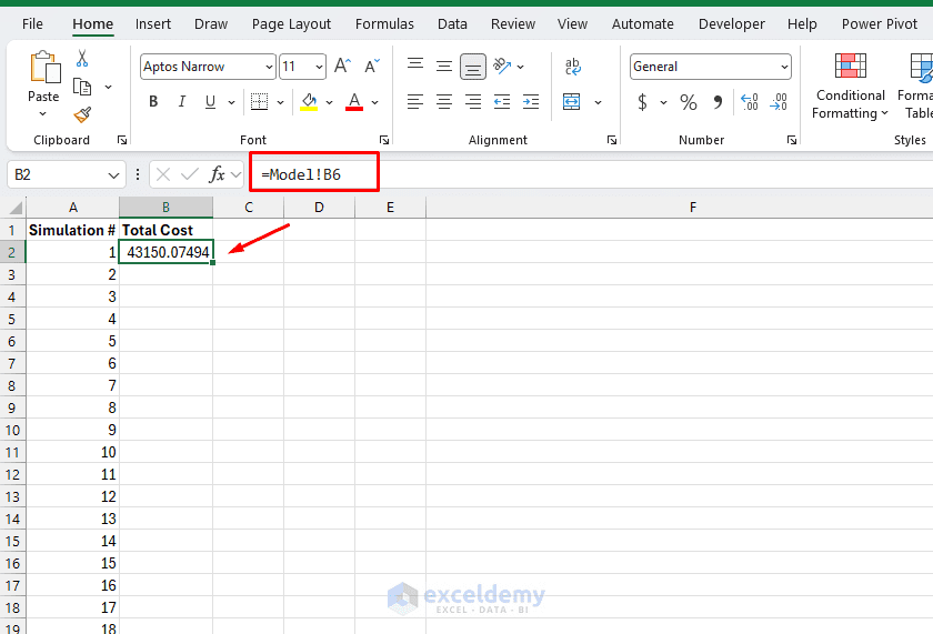
• In cell B2, link to your output cell:

=Model!B6

Execute the Simulation:

• Select the range A2:B10001
• Go to the Data tab >> select What-If Analysis >> select Data Table
  • Leave the Row input cell blank
  • Set the Column input cell to any empty cell (e.g. S1) — this forces recalculation on each row
  • Click OK

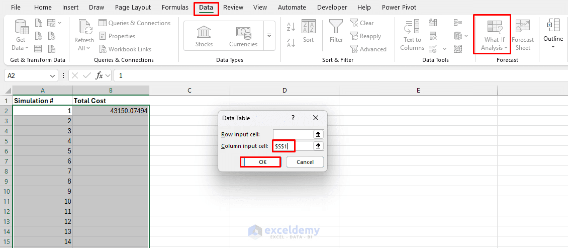
Excel will fill Column B with 10,000 different Total Cost values as the RAND functions recalculate per row. Press F9 to refresh the entire simulation.

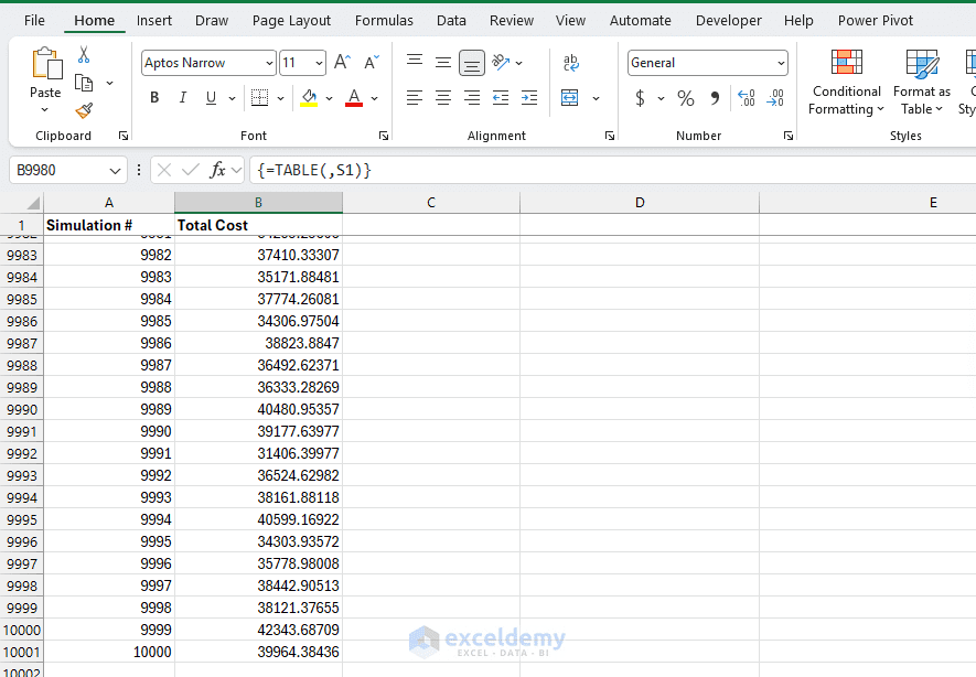
Important Settings:

• Switch to Manual Calculation:
  • Go to the Formulas tab >> select Calculation Options >> select Manual
• Press F9 to generate a new set of simulations
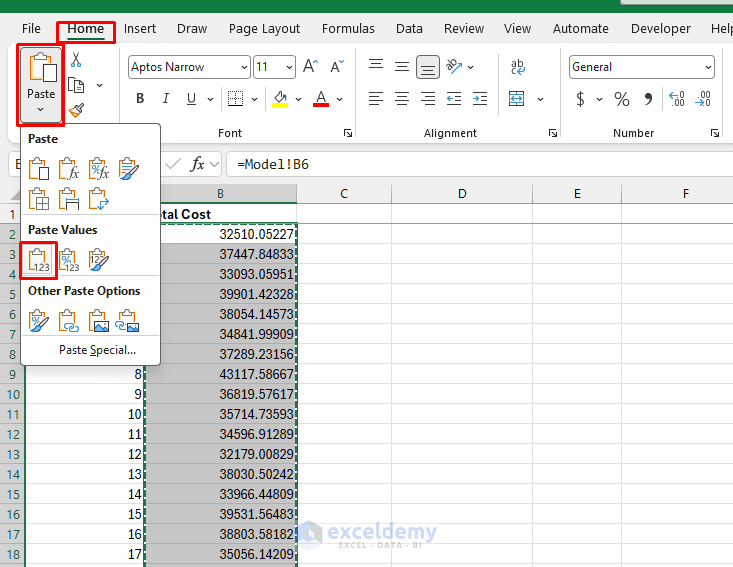
• After getting results:
  • Select Column B and Copy it
  • Select Paste Special >> select Values (to freeze the numbers)

Step 3: Statistical Analysis and Interpretation in Excel

Add summary statistics below the table:

• Mean:

=AVERAGE(B3:B10002)

• Median:

=MEDIAN(B3:B10002)

• Std Dev:

=STDEV.S(B3:B10002)

• Percentile (P10):

=PERCENTILE.INC(B3:B10002,0.1)

• Percentile (P50):

=PERCENTILE.INC(B3:B10002,0.5)

• Percentile (P90):

=PERCENTILE.INC(B3:B10002,0.9)

• Probability of overrun > 45,000:

=COUNTIF(B3:B10002,">45000")/10000

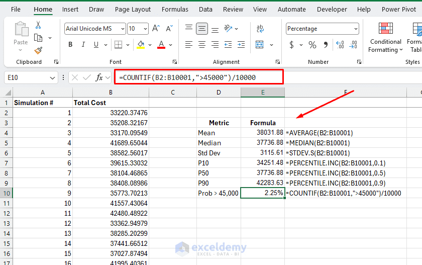
This gives you empirical probability distributions.

Key Interpretation Examples:

• There is approximately a 2.25% chance the project will cost more than $45,000
• To be 90% confident, budget around $42,283.63
• The average simulated cost ($38,031.88) is higher than the deterministic estimate because of the positive skew in the distributions

Step 4: Analyze Distributions Statistically in Excel

You can use the built-in tools or Excel formulas to analyze distributions statistically.

Analysis ToolPak (Recommended):

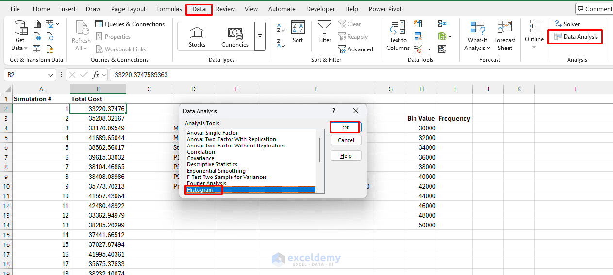
• Go to the Data tab >> select Data Analysis >> select Histogram
• Click OK

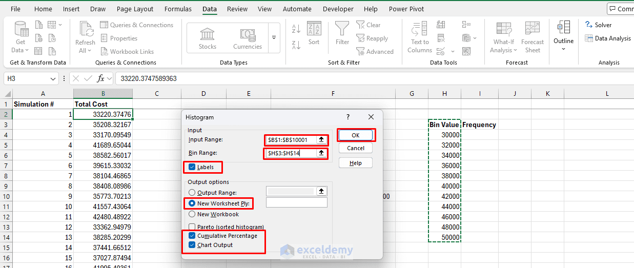
• In the Histogram dialog box, enter the following:
  • Input Range: B1:B10001
  • Bin Range: H13:H14 (or leave it empty to use automatic bins)
  • Check Labels
  • Check Cumulative Percentage
  • Check Chart Output
  • Select New Worksheet as the output location
  • Click OK

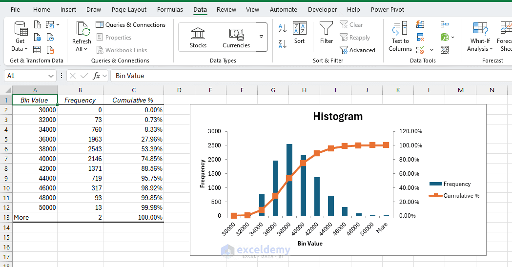
• You will get the frequency table along with a histogram chart

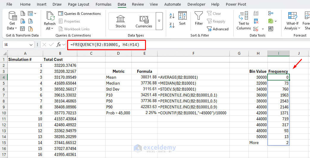
FREQUENCY Function:

• Create the bin list
• Insert the following formula:

=FREQUENCY(B2:B10001, H4:H14)

• Go to the Insert tab >> select Histogram
• Set Gap Width to 0%
• Add the chart title: "Total Project Cost Distribution – 10,000 Simulations"
• Label the axes appropriately

Step 5: Visualization and Interactivity in Power BI

Export the frozen simulation results (Simulation # and Total Cost columns) as a table or CSV, then load them into Power BI.

Import Data:

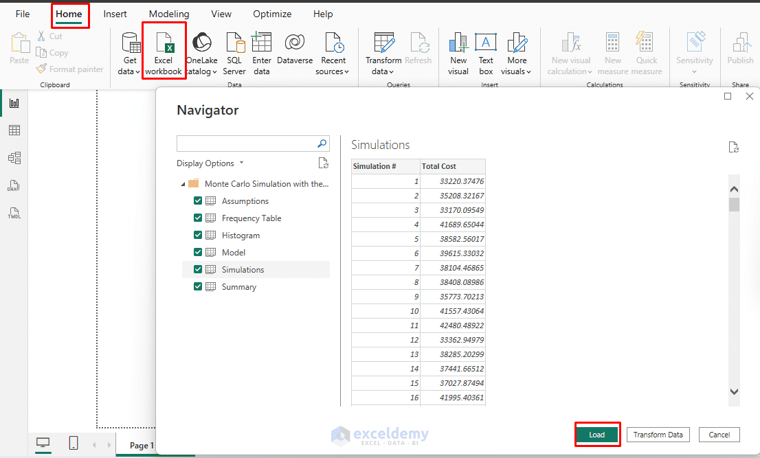
• Go to the Home tab >> select Excel Workbook
• Browse and select your file
• Select the Simulations sheet
• Click Load to import the data directly into Power BI

Power BI Modeling and Visuals:

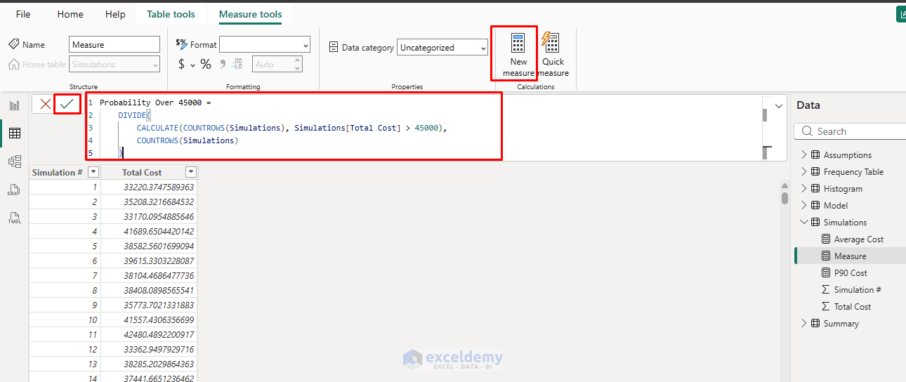
• Create the following Measures:

Average Cost = AVERAGE(Simulations[Total Cost])

P90 Cost = PERCENTILE.INC(Simulations[Total Cost], 0.9)

Probability Over 45000 =
DIVIDE(
CALCULATE(COUNTROWS(Simulations), Simulations[Total Cost] > 45000),
COUNTROWS(Simulations)
)

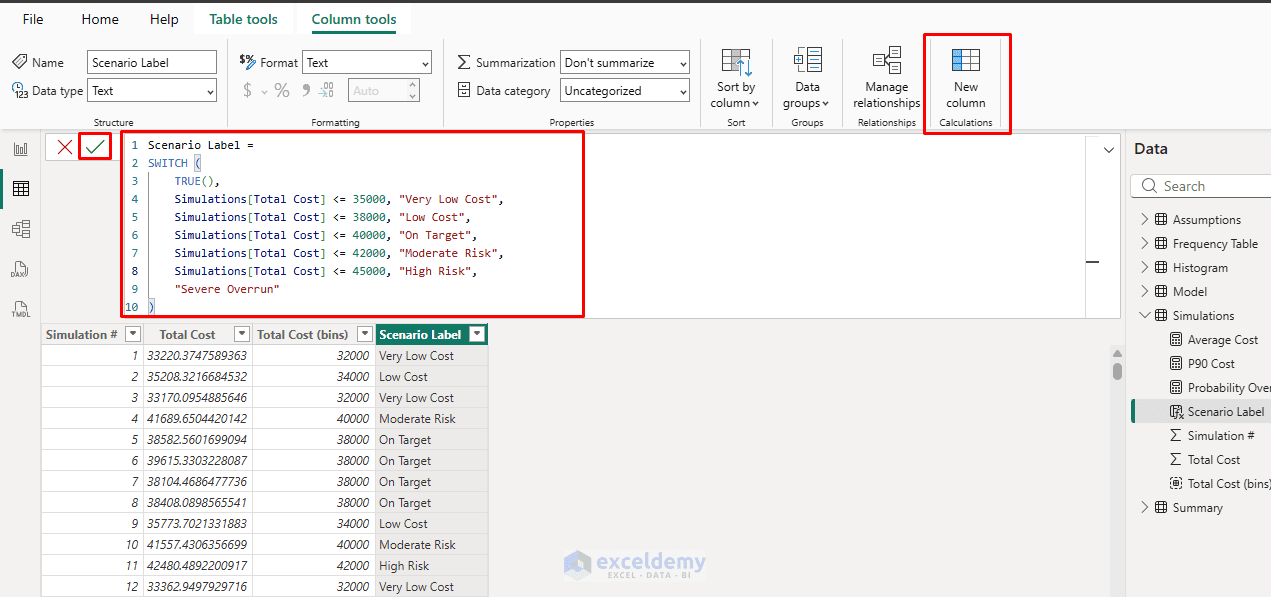
• Create the following new calculated column to generate scenario labels:

Scenario Label =
SWITCH (
TRUE(),
Simulations[Total Cost] <= 35000, "Very Low Cost",
Simulations[Total Cost] <= 38000, "Low Cost",
Simulations[Total Cost] <= 40000, "On Target",
Simulations[Total Cost] <= 42000, "Moderate Risk",
Simulations[Total Cost] <= 45000, "High Risk",
"Severe Overrun"
)

Key Visualizations:

• Histogram: Show Total Costs (use bin grouping on a visual)
• Line Chart: Cumulative Distribution Function (CDF)
• KPI Cards: Avg Cost, P90 Cost, Probability of Overrun
• Table: Show the summary statistics
• Slicers: For scenario filtering

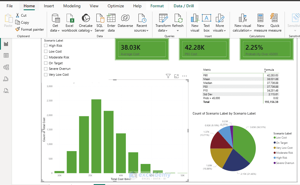
Power BI makes the report interactive: users can adjust target budgets and instantly see the resulting probabilities.

Step 6: Communicate in PowerPoint

Turn insights into a compelling story:

• Slide 1: Problem and Deterministic vs. Probabilistic View (single number vs. distribution).
• Slide 2: Key Assumptions and Distributions (show input triangles/normals).
• Slide 3: Simulation Setup (screenshot of the Excel model + "10,000 iterations").
• Slide 4: Results Dashboard (embed or screenshot Power BI visuals).
  • "Mean total cost: $XXk (vs. deterministic $YYk)"
  • "15% chance of exceeding $ZZk budget"
• Slide 5: Sensitivity/Tornado chart (from additional Excel tables).
• Slide 6: Recommendations and Decision Framework (e.g. "Add 20% contingency for 90% confidence")

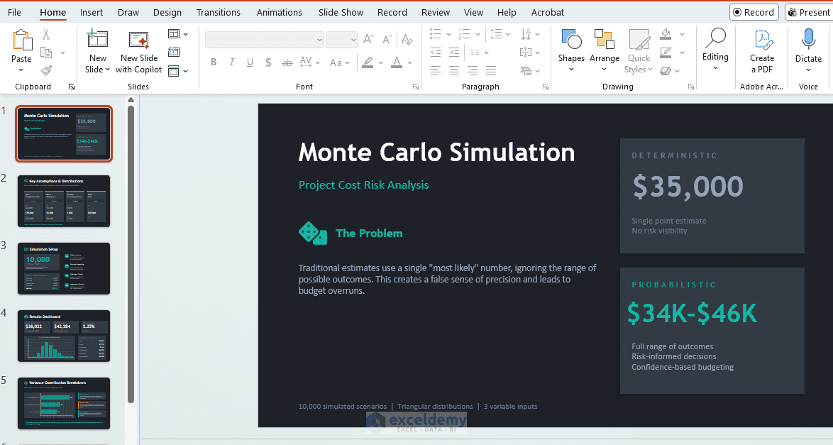
Tip: If you have access to Copilot, you can use the Excel file or Power BI report to generate your presentation quickly and easily.

Best Practices for Slides:

• Use clear, quantified titles like "Probability of On-Time Delivery: 72%"
• "We are 90% confident the project cost will not exceed $42,100."
• "There is only a 3% probability of severe overrun (> $45k)."
• Include confidence intervals or percentile ranges
• Avoid clutter — one key visual per slide
• Add a "How We Did This" appendix for transparency

Limitations and Statistical Rigor Notes

• Excel's RAND() is pseudo-random but sufficient for most business applications (use RANDARRAY in newer Excel versions for better efficiency)
• 5,000–10,000+ iterations are recommended for stable results
• Document your random seed approach (or note the lack of reproducibility without VBA)
• Always validate against known analytical solutions where possible (e.g. simple sum of normals)
• Be transparent about assumptions — Monte Carlo is only as good as your input distributions

Conclusion

Monte Carlo simulation helps decision-makers understand uncertainty instead of obscuring it behind a single fixed forecast. With the Microsoft Stack, the full process can be completed without writing any code. Excel generates thousands of random scenarios, Power BI visualizes the probability distribution, and PowerPoint communicates the results in a way that supports better decisions. This approach empowers analysts, managers, and decision-makers to move from gut feel to quantified risk using tools they already have. Start small with one uncertain variable, scale up, and iterate.