Latest Posts From Shamima Sultana

In this tutorial, we will show how to use Power BI Dataflows to create reusable ETL (Extract, Transform, Load) for your Excel and Power BI reports. Instead of ...

In this tutorial, we will show how you can visualize Excel data with ChatGPT, from getting smart chart-type recommendations based on your data structure to ...

In this tutorial, we will show five Excel functions that every marketer should know. These functions can help you summarize, categorize, measure campaign ...

In this article, we have listed the top 10 Excel influencers you can follow on YouTube. These Excel influencers consistently publish high-quality content, ...

In this tutorial, we will show how to connect Excel to live web APIs without using VBA. We will use Power Query’s From Web feature to pull live API data into ...

In this tutorial, we will show 5 LAMBDA functions that turn Excel into your own programming language.

In this tutorial, we will show how to fix Excel formulas with ChatGPT. ChatGPT excels as a debugging partner: it can explain complex formulas, diagnose issues, ...

In this tutorial, we will show how to use Boolean variables in VBA. Instead of writing long conditions repeatedly, you can store the result in a Boolean ...

In this tutorial, we will show how to rename visual fields without changing your Power BI source data. At the same time, keep the data model intact.

In this tutorial, we will show how to use conditional formatting in Power BI for table cell colors.

In this tutorial, we will show how you can mine your Excel spreadsheets with ChatGPT. You will get the prompts and techniques to get actionable insights ...

In this tutorial, we will show how to format dates in Excel using VBA. Here you will get VBA examples with short codes.

In this tutorial, we will show how to build an automated invoice routing workflow with Excel and Power Automate. It will read new invoice rows from Excel, send ...

In this tutorial, we will show how to build Excel spreadsheets with ChatGPT. Let’s explore how to use ChatGPT to create Excel spreadsheets faster and more ...

In this tutorial, we will show how to build 5 dynamic Excel templates for start-up financial projections. These templates will help startups track cash flow, ...
- 1
- 2
- 3
- …
- 26
- Next Page »
See Our Reviews at


Hi Arda
Hope you are doing well.
I checked the code you mentioned above and it works. To make it more clear I’m attaching some images with the code.
Here, I tried the exact code in the same dataset.
MsgBox Range("E5").End(xlToRight).Offset(0, 1).AddressYou can see the result $G$5.
Again I changed the dataset slightly.
Here, the result is also based on the location.
NB. If it doesn’t help you then please send your dataset to [email protected] or [email protected]
Thanks
Shamima Sultana
ExcelDemy
Hello,
You are most welcome. Thanks for your feedback and appreciation. Glad to hear that our post is helpful to you.
Regards
ExcelDemy
Hello Chantra,
You’re very welcome! Thank you for your suggestion. A template that supports multiple shift patterns (24-hour, 12-hour, 8-hour, Monday–Friday, weekends, holidays, and custom rotations) would require a more advanced design than the one covered in this article, so we don’t have a ready-made version available at the moment.
We’ll certainly consider creating a dedicated template for this type of healthcare roster in a future article. Thank you for the great idea!
Best regards,
ExcelDemy
Hello Anakin,
The restriction is optional and is created only when the worksheet’s ScrollArea property is set. Setting it to A1:H15 means that cells inside A1 can be selected, while cells outside that range cannot be selected.
To remove the restriction, open the worksheet’s Properties window in the VBA Editor and clear the value from the ScrollArea field. You will then be able to select all cells normally.
Regards,
ExcelDemy
Hello Chantra,
You can create this healthcare roster by adding a Schedule Type column beside each employee’s name. For example, enter 24H, 12H, 8H, or MON-FRI.
Assume:
1. Employee names are in column B.
2. Schedule types are in column C.
3. The employee’s rotation start date is in column D.
4. Roster dates begin in cell E7.
5. The first employee’s schedule begins in E8.
You can enter the following formula in E8 and drag it across and down:
=IF(E$7=””,””,SWITCH($C8,
“24H”,IF(MOD(E$7-$D8,2)=0,”24H”,”REST”),
“12H”,INDEX({“DAY 12H”,”NIGHT 12H”,”REST”,”REST”},MOD(E$7-$D8,4)+1),
“8H”,INDEX({“DAY 8H”,”DAY 8H”,”DAY 8H”,”DAY 8H”,”DAY 8H”,”REST”,”REST”},MOD(E$7-$D8,7)+1),
“MON-FRI”,IF(OR(WEEKDAY(E$7,2)>5,COUNTIF(Holidays,E$7)>0),”OFF”,”DAY 8H”),
“”))
Here, Holidays should be a named range containing your organization’s holiday dates. This example assigns:
1. 24-hour duty followed by one rest day.
2. A 12-hour day shift, a 12-hour night shift, and two rest days.
3. Five 8-hour duty days followed by two rest days.
4. Monday-to-Friday duty with weekends and listed holidays off.
You can also calculate each employee’s total scheduled hours with:
=COUNTIF(E8:AI8,”24H”)*24+(COUNTIF(E8:AI8,”DAY 12H”)+COUNTIF(E8:AI8,”NIGHT 12H”))*12+COUNTIF(E8:AI8,”*8H”)*8
These are sample rotation rules. You may modify the sequence inside the formula according to your hospital’s actual duty, rest, weekend, and holiday policies.
Best regards,
ExcelDemy
Hello Michael Beck,
Thank you for explaining the issue. Using 14N and 14R produces the same result because the VBA code uses the letter only to determine whether the location is in the Northern or Southern Hemisphere.
The more likely issue is that your original Easting and Northing values are not actually UTM coordinates. Many North Texas surveys and maps use NAD83 Texas State Plane North Central coordinates, often measured in US survey feet. Converting those values to meters is not enough because State Plane and UTM use different projections.
Please check the coordinate-system information on the original map or data file. If it states something such as Texas North Central, NAD83, FIPS 4202, State Plane, or EPSG:2276, the coordinates must first be reprojected to WGS84 / UTM Zone 14N before using this VBA function.
For reference, valid UTM coordinates around the Dallas–Fort Worth area are generally approximately 500,000–750,000 meters Easting and 3,500,000–3,800,000 meters Northing. You may also share one sample Easting/Northing pair and the exact datum or coordinate system so we can identify the required conversion.
Regards,
ExcelDemy
Hello Acarolinensis,
You are most welcome. Thanks for your detail feedback and appreciation. Glad to hear that you liked the solution.
Keep exploring Excel with ExcelDemy!
Regards,
ExcelDemy
Hello Deepankar,
You are most welcome. Thanks for your appreciation.
Keep exploring Excel with ExcelDemy!
Regards,
ExcelDemy
Hello Chioma,
You are most welcome. We have prepared a sample loan dataset that you can use to calculate Days Past Due and monthly roll rates. It includes Account ID, snapshot date, oldest unpaid due date, scheduled payment, amount paid, outstanding balance, DPD bucket, and month-to-month transitions.
You can download the sample dataset and use the included formulas and Roll Rate sheet for practice. Please let us know if you need any additional help.
Loan Roll Rate DPD Sample Dataset.xlsx
Regards,
ExcelDemy
Hello Willie Mukar,
Thanks for your feedback and appreciation. Glad to hear that our tutorial made your job easy.
Keep exploring Excel with ExcelDemy to get such helpful content more.
Regards,
Exceldemy
Hello Shou Mau,
You can remove all #NUM! errors at once using Find and Replace:
1. Press Ctrl + H.
2. In Find what, enter #NUM!.
3. Leave Replace with blank.
4. Click Options and set Look in to Values.
5. Click Replace All.
Please note that this only removes the displayed error values; if the errors are produced by formulas, it may be better to correct the formulas or wrap them with IFERROR, for example: =IFERROR(your_formula,””).
Regards,
ExcelDemy
Hello Baabu,
Thanks for your feedback and appreciation. Glad to hear that you liked our template and it is easy to use.
Keep exploring Excel with ExcelDemy!
Regards,
ExcelDemy
Hello Bob Dragon,
Thank you for the thoughtful feedback. You make a valid point—the article should explain not only how each method works, but also how practical and maintainable it is when the source list changes.
The CHOOSE and RANDBETWEEN method is included mainly to demonstrate another possible approach. However, we agree that manually listing every cell makes it unsuitable for a growing or frequently changing list. In most cases, the INDEX formula using ROWS is a much better option:
=INDEX(B5:B12,RANDBETWEEN(1,ROWS(B5:B12)))
For even greater flexibility, the source data can be converted into an Excel Table so that the formula automatically adjusts when items are added or removed. We appreciate your suggestion and will consider adding a comparison of the methods and their limitations to make the article more useful.
Regards,
ExcelDemy
Hello Manuel,
Thank you so much for your kind words! We’re delighted to hear that you liked our Excels support.
Regards,
ExcelDemy
Hello Dr. Ronal J. Tuman,
Thank you so much for your kind words! We’re delighted to hear that the instructions were clear and helpful, especially as you’re new to VBA. It’s great to know you successfully created a similar workbook using VBA and bookmarks.
Regards,
ExcelDemy
Hello Abdul Kader,
Thank you for your feedback. We’re glad to hear Method 3 is working for you. Regarding the VLOOKUP issue, it usually happens when the table range or lookup references are not locked correctly. When copying the formula down, make sure the lookup table range is fixed with absolute references (using $ signs), while the lookup value reference remains relative. For example:
=VLOOKUP(B17,$H$2:$J$100,2,FALSE)
When you drag this formula down, B17 will change to B18, B19, etc., but the lookup table range will remain unchanged.
If this doesn’t resolve the issue, could you share the exact VLOOKUP formula you’re using and a brief description of your data layout? We’d be happy to help further.
Regards,
ExcelDemy
Hello Ed Eaglehouse,
Thank you for sharing your feedback. You’re right that Excel has a limitation when it comes to automatically adjusting row height for merged cells with wrapped text. Unfortunately, this behavior is built into Excel itself and isn’t something that can be fully controlled through standard formatting options. We appreciate your comment and understand how frustrating this limitation can be when working with merged cells.
Regards,
ExcelDemy
Hello Peter S,
Thank you for catching this. You were right that the formula shown in Method 2 contained an error. We’ve corrected the formula and removed the unintended expression that appeared after the second SUMIF function. We appreciate your careful review and feedback, which helped us improve the accuracy of the article.
Regards,
ExcelDemy
Hello Peter S,
Thank you for pointing this out. Method 2 double-counted records that met both criteria, which led to the incorrect total of 48,650. We have updated the article and revised the method to apply OR logic without double-counting overlapping records. The corrected result is now 39,084. We appreciate your careful review and feedback!
Regards,
ExcelDemy
Hello Peter S.,
Thank you for catching that. You were right—the original example could lead to double-counting. We’ve reviewed and corrected the example in the article to address the issue. We appreciate your feedback, as it helps us improve the accuracy of our content.
Regards,
ExcelDemy
Hello Fer,
Thank you for your comment. IMEXP() is indeed another important function in Excel’s Complex Number category. This article covers many of the commonly used complex functions, but not every function available in the category. We appreciate your feedback and will consider adding IMEXP() in a future update to make the resource more comprehensive.
Regards,
ExcelDemy
Hello Danniell,
Thank you for your feedback. The formula in the article calculates the straight-line (great-circle) distance between two cities based on their latitude and longitude coordinates. Google Maps, however, typically shows driving distance, which follows roads, highways, and route restrictions.
Because of this difference, the Excel result may be significantly lower or higher than the distance shown in Google Maps. Please make sure that the latitude and longitude values are entered correctly and that the same unit (miles or kilometers) is being used throughout the calculation.
If you need driving distance rather than straight-line distance, you would need to use a mapping service such as Google Maps or an API that calculates road routes.
Regards,
ExcelDemy
Hello Catherine,
You are most welcome. Thanks for your feedback and appreciation. Glad to hear that you like our article and it saved your precious time.
Regards
ExcelDemy
Hello Imran Malik,
Thank you for your comment. The article provides a customizable labor contractor bill format that you can modify for use between a manufacturing company and a labor contractor. Simply download the template and edit the company details, contractor information, labor charges, attendance records, and payment details according to your requirements.
Regards,
ExcelDemy
Hello Alen,
It was a linking issue. It is resolved now. Please check the file now.
Regards,
ExcelDemy
Hello Alen,
Here, I am attaching the data file to practice by yourself.
Download it from here: 3 Dynamic Array Formulas That Make Your Old Workbooks Look Like Antiques.xlsx
Regards,
ExcelDemy
Hello Abdelmutaal,
Please check now, article itself was linked instead of the Excel file.
Regards,
ExcelDemy
Hello Alex,
This usually happens when the horizontal axis values are entered as actual percentages instead of whole-number axis values.
For this Mekko chart method, please enter the horizontal axis values as numbers such as `0`, `20`, `55`, `100`, etc. Then apply the custom number format:
`0″%”`
Do not enter them as `0%`, `20%`, `55%`, etc., because Excel stores those as decimal values like `0`, `0.2`, and `0.55`. When you later change the horizontal axis to a Date Axis, those very small values can make the chart sections collapse together and appear like one column.
After correcting the helper axis values, format the horizontal axis again as a Date Axis and set the Major and Minor Units to 10.
Regards,
ExcelDemy
Hello Tim,
Yes, you can apply the same tab setup to multiple sheets by looping through the worksheets in VBA instead of writing the code for only one sheet.
For example, if the same shapes and columns exist on every sheet, you can use code like this:
You can modify the same way for the other tab macros. Just make sure that every worksheet has the same shape names, such as EplOn, EplOff, BundOn, BundOff, etc. Otherwise, VBA will show an error.
If you want to apply it only to selected sheets, use this structure:
For Each ws In Sheets(Array(“Sheet1”, “Sheet2”, “Sheet3”))
instead of:
For Each ws In ThisWorkbook.Worksheets
Regards,
ExcelDemy
Hello Kim,
This usually happens because of a slight page setup, scaling, or printer alignment issue rather than the Excel data itself. Please check the following:
1. Make sure you selected Avery US Letter and 5160 Address Labels in Word.
2. In the Print settings, set scaling to Actual Size / 100%. Do not use Fit to Page or Scale to Fit.
3. Confirm the paper size is Letter, not A4.
4. Print a test page on plain paper first and place it behind the Avery sheet to check the alignment.
5. If only the third row is slightly shifted, you can adjust the label layout from Mailings > Labels > Options > Details and slightly modify the vertical pitch/top margin.
This type of issue often depends on the printer’s margin handling, so a small adjustment in Word’s label details usually fixes it.
Regards,
ExcelDemy
Hello Abdelmutaal,
You are most welcome. Thanks for your feedback and appreciation. Here, I am attaching the Excel file. Download it to practice and make it your own.
5 Dynamic Excel Templates for Start-up Financial Projections.xlsx
Regards,
ExcelDemy
Hello Usman,
Here, I am attaching the Excel file. Download it to practice and make it your own.
5 Dynamic Excel Templates for Start-up Financial Projections.xlsx
Regards,
ExcelDemy
Hello Pla,
Thank you for pointing this out. In Example 7, the average range needs to be locked to keep the Advanced Filter result accurate.
We have updated the formula to:
=$G5>AVERAGE($G$5:$G$23)
Here, $G5 checks each row’s price, while $G$5:$G$23 keeps the average range fixed. Thanks again for your careful observation and helpful feedback.
Regards,
ExcelDemy
Hello Jejo,
You are most welcome. Thanks for your kind words. Glad to hear that you liked our tutorial.
Keep exploring Excel with ExcelDemy!
Regards,
ExcelDemy
Hello Nilesh Chauhan,
You can certainly add another worksheet for data entry. Simply create a new sheet and use the same layout as the existing data entry sheet. This can be helpful if you want to separate different types of data or keep records for different periods.
Regards,
ExcelDemy
Hello Stephen,
I’m glad you were able to get the formula working! Yes, the fraction can be rounded to a specific denominator such as 1/16″ or 1/32″. The formula I provided uses Excel’s default fractional formatting, which may return values such as 5 2/3″ rather than the construction-style fractions commonly used in industry.
For example, to round the inch portion to the nearest 1/16″, you can first round the value:
=ROUND(C5*16,0)/16
and then convert the result to feet and inches.
For your example of 2777.689″, rounding to the nearest 1/16″ would give a result closer to the format typically used in construction, woodworking, and manufacturing applications.
As for having to post twice, that is likely related to the website’s moderation or approval process rather than anything in Excel.
Thank you for testing the formulas and providing feedback. I’ll see if I can come up with a cleaner single-cell formula that always returns feet and inches rounded to a specified fraction such as 1/16″ or 1/32″.
Regards,
ExcelDemy
Hello Sudhakar,
Absolutely! If you’re just getting started with Excel, we have a complete learning hub that covers everything from beginner to advanced topics:
https://www.exceldemy.com/learn-excel/
You may also find these categories helpful:
• Excel Basics: https://www.exceldemy.com/topics/excel-basics/
• Excel Formulas & Functions: https://www.exceldemy.com/topics/excel-formulas/
• Excel Charts: https://www.exceldemy.com/topics/excel-chart/
• Excel VBA & Macros: https://www.exceldemy.com/topics/excel-vba/
• Advanced Excel: https://www.exceldemy.com/topics/advanced-excel/
We recommend starting with the Excel Basics section and then moving on to formulas, functions, and data analysis as you become more comfortable.
Happy learning, and feel free to ask if you have any specific Excel questions!
Regards,
ExcelDemy
Hello Creavis Meult,
Excel has a fixed column limit. A single worksheet can contain only 16,384 columns, ending at column XFD. So, 837,281 columns cannot fit in one Excel sheet.
If you actually mean 837,281 rows, then it can fit, because Excel supports up to 1,048,576 rows per worksheet.
For 837,281 columns, you may need to restructure the data, split it across multiple sheets/files, or use a database/Power Query/Power Pivot depending on your purpose.
Regards,
ExcelDemy
Hello Stephen,
Thank you for checking again. Please try this simpler formula:
=TEXT(C5/12,”#’ ?/12″)
However, for the exact format 1′ 7 1/8″, this formula should work better:
=INT(C5/12)&”‘ “&TEXT(MOD(C5,12),”# ?/?”)&””””
If Excel still shows a punctuation error, please manually replace the last part &”””” by typing four double quotation marks from your keyboard. Sometimes copied quotation marks from web comments become “smart quotes,” and Excel cannot read them.
Regards,
ExcelDemy
Hello David,
You can download the file from the download section, given in the bottom section of the article.
Here, I am attaching it for you: Mortgage Calculator with Extra Payments and Lump Sum in Excel.xlsx
Regards,
ExcelDemy
Hello A,
Thank you for sharing the issue. This usually happens when Excel treats the selected range as plain text or when the chart is inserted from a text box/shape instead of the actual data range.
Please try the following:
1. Make sure your data is arranged in two separate columns: one column for the words/categories and another column for the values.
2. Select the actual cell range, not a text box.
3. Go to the Insert tab >> select Pie Chart and choose a 2-D Pie Chart.
4. If you still see text inside the chart area, right-click the chart and choose Select Data, then manually select the correct data range.
Also, make sure the value column contains numbers, not numbers stored as text. You can test this by selecting the value cells and changing the format to Number.
If the problem continues, please share a screenshot of your data range and the chart area so we can identify the exact issue.
Regards,
ExcelDemy
Hello Usman,
Here, I am attaching the data file to practice by yourself.
Download it from here: 3 Dynamic Array Formulas That Make Your Old Workbooks Look Like Antiques.xlsx
Regards,
ExcelDemy
Hello Stephen,
Thank you for letting me know. The issue is likely due to the quotation marks being converted when copied from the website or comment section.
Please try typing the formula directly into Excel rather than copying it from the comment.
You can also try this version:
=INT(C5/12)&”‘ “&TEXT(MOD(C5,12),”# ?/?”)&””””
For a value of 19.125 in C5, the result should be: 1’ 7 1/8″
If you still receive an error, could you please let me know:
1. Your Excel version (Excel 365, 2021, 2019, etc.)
2. Whether your formulas use commas (,) or semicolons (;)
That will help me provide the exact formula for your setup.
Regards,
ExcelDemy
Hello Stephen,
Thank you for your kind words. To convert a decimal inch value like 19.125 into 1′ 7 1/8″, you need to convert the decimal part of the inches into a fraction.
You can use this formula:
=INT(C5/12)&”‘ “&INT(MOD(C5,12))&” “&TEXT(MOD(C5,1),”# ?/?”)&””””
For 19.125, this returns: 1′ 7 1/8″
Here, INT(C5/12) returns the feet, INT(MOD(C5,12)) returns the whole inches, and TEXT(MOD(C5,1),”# ?/?”) converts the decimal inch part into a fraction.
Regards,
ExcelDemy
Hello Mohaimen,
Walaikumassalam, hope you are doing well. We have video tutorial in youtube, you can explore our Youtube chanel:
Regards,
ExcelDemy
Hello Desain Kreatif,
Thank you so much for your kind feedback! We’re glad to know that the sample datasets are helping you practice Power Query and data cleaning more effectively. Multi-row and less “clean” datasets are especially useful for building real-world Excel skills, so it’s great to hear that you found the variety helpful. Stay connected with ExcelDemy for more practical datasets and tutorials.
Regards,
ExcelDemy
Hello Niraj Man,
You are most welcome. Thanks for your suggestion. Of course, you can simplify long formula with existing updated dynamic formulas. We appreciate your feedback. Glad to hear that you learnt a lot from our tutorial.
Regards,
ExcelDemy
Hello Ei,
This article provides an Excel-based chart of accounts template for a construction company, which can help you organize income, expenses, assets, liabilities, and project-related accounts.
If you are looking for full construction accounting software, you may consider software that supports job costing, project budgeting, invoicing, payroll, vendor payments, and financial reporting. You can also use our Excel template as a starting point before moving to dedicated construction accounting software.
Regards,
ExcelDemy
Hello Ernie Thackeray,
Thank you for your feedback. Only the location image may not fully meet the requirement if you want the city names displayed directly on the map.
In Excel, the built-in Map Chart mainly plots locations based on geographic data, but city name labels may not always appear clearly or automatically. To show city names, you can try enabling Data Labels from the Chart Elements option. If that does not work as expected, using 3D Maps is usually a better option because it provides more control over location labels and map visualization.
Reggards,
ExcelDemy
Hello Mohammed Nadim,
Thanks for your feedback and appreciation. Your feedback is so amazing and constructive. Glad to hear that you the breakdown is helpful to choos ethe right function. If you need further help, please let us know.
Regards,
ExcelDemy
Hello Kalai,
Thanks for your feedback and appreciation. Glad to hear that you liked our explanation and clarity.
Regards,
ExcelDemy
Hello Haro,
You are most welcome. Glad to hear that our datasets are helping our users.
Keep exploring Excel with ExcelDemy!
Regards,
ExcelDemy
Hi Roopasri,
If you need any help regarding Excel, feel fre to post here.
We are here to help you.
Regards,
ExcelDemy
Hello Usman,
Here, I am attaching the data file tp practice more efficiently.
Download the file from here: How to Create and Summarize Pivot Tables in Excel Using Copilot
Regards,
ExcelDemy
Hello Rahat,
Thanks for your feedback and appreciation. Glad to heart that our article helped you to do the speed comparison in minutes.
Keep exploring Excel with ExcelDemy!
Regards,
ExcelDemy
Hello Amit Kumar,
Thank you for your feedback. The article covers several examples step by step, but some parts can feel difficult if you are new to Decision Trees or machine learning in Excel. Please let us know which section was confusing, and we’ll try to explain it more clearly for you.
Regards,
ExcelDemy
Hello Kelly,
Custom number formatting in Excel can display fixed text, but it can’t enforce alphabetic character input like requiring “AB” at the beginning. Custom formats mainly control how values appear after entry.
For a pattern like “AB12-345-67”, the better approach is usually:
• Data Validation to control the allowed structure
• Or VBA for stricter letter/number enforcement
For example, you could use a custom format to display separators:
00-000-00
Solution:
You can’t force letters using Custom Number Format alone. For a value like AB12-345-67, use Data Validation instead.
Select the input cells, then go to Data > Data Validation > Custom and use this formula, assuming the first cell is A1:
=AND(LEN(A1)=11,COUNT(FIND(MID(UPPER(LEFT(A1,2)),{1,2},1),”ABCDEFGHIJKLMNOPQRSTUVWXYZ”))=2,MID(A1,5,1)=”-“,MID(A1,9,1)=”-“,COUNT(FIND(MID(A1,{3,4,6,7,8,10,11},1),”0123456789”))=7)
This will allow entries like: AB12-345-67
And reject entries where the first two characters are not letters, the hyphens are missing, or the number positions are invalid.
Regards,
ExcelDemy
Hello Rhoda,
Thank you so much for your kind feedback! We’re really glad you found the document useful.
You can start learning Excel from our organized tutorial categories and free courses:
Excel Learning Hub: https://www.exceldemy.com/learn-excel/
Excel Basics: https://www.exceldemy.com/topics/excel-basics/
Advanced Excel: https://www.exceldemy.com/topics/advanced-excel/
Our tutorial categories include:
and many more practical Excel topics with step-by-step explanations and practice files.
Happy learning with ExcelDemy!
Regards,
ExcelDemy
Hello Nick,
Thank you so much for your detailed input! Really appreciate you pointing out these edge cases.
Your suggestions for handling numbers between 0 and 1 (Deg = Int(Round(Decimal_Degrees, 0))) and negatives (Min = Abs(Decimal_Degrees – Deg) * 60) make the VB code much more accurate and reliable. This kind of feedback is incredibly helpful!
Regards,
ExcelDemy
Hello David Snipes,
Thanks for your appreciation and feedback. Glad to hear that you liked our article.
Keep exploring Excel with ExcelDemy!
Regards,
ExcelDemy
Hello Rajeswri Chowdhury,
You are most welcome. Thanks for your appreciation and feedback. Glad to hear that our sample datasets are helping learners to practice advanced Excel and data analysis.
Keep exploring Excel with ExcelDemy!
Regards,
ExcelDemy
Hello Jorge,
Hello, I’m sorry you’re still having trouble. If you’ve already tried reinstalling Office and it’s not working, it might help to try a few other solutions. Make sure your Office is updated to the latest version. You could also try temporarily disabling your antivirus to see if it’s causing any conflicts. If the issue persists, I would recommend reaching out to Microsoft’s support for more specific assistance. Hope it gets resolved soon!
Regards,
ExcelDemy
Hello Clive Emberey,
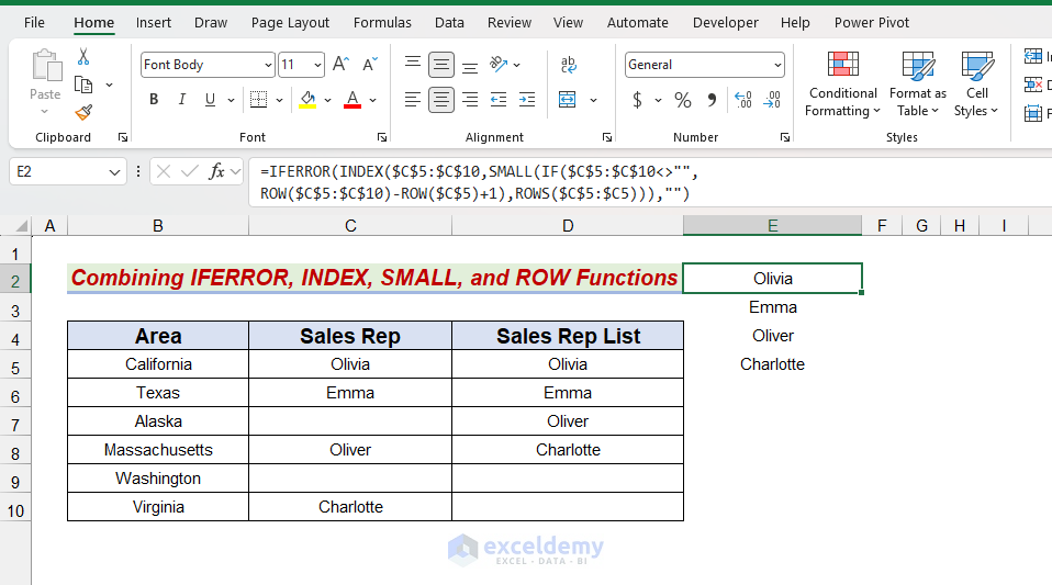
Thank you for your detailed feedback. We reviewed and tested Method 2 again. The formula works correctly when the output starts in the intended first output cell. However, we understand that the ROWS($C$5:$C5) counter can be confusing if readers place the formula in a different row without adjusting the reference. We have updated the explanation to make this clearer. You were also right that the note should refer to IFERROR, not ISERROR, and we have corrected that. Thanks again for helping us improve the article.
Regards,
ExcelDemy
Hello Satarrah,
Yes, you can show the annual leave balance in hours instead of days by converting the day-based result into hours.
For example, if your leave balance is calculated in days and one working day equals 8 hours, you can use:
=Leave_Days*8
So, if the remaining leave is in cell G2, use:
=G2*8
Then change the column header from Remaining Leave (Days) to Remaining Leave (Hours).
If your company uses a different daily working hour, such as 7.5 hours, use:
=G2*7.5
You can also modify the main leave calculation formula directly by multiplying the final result by the number of working hours per day.
Regards,
ExcelDemy
Hello Mose Hurt,
You are most welcome. Thanks for your appreciation. We are glad to hear that our article helped you to understand anchoring easily.
Keep exploring Excel with ExcelDemy!
Regards,
ExcelDemy
Hello Mohammad Hossain,
You are most welcome. Thanks for your appreciation an feedback. Glad to hear that our article helped you to create a student result sheet.
Keep exploring Excel with ExcelDemy!
Regards,
ExcelDemy
Hello Eddie,
You are most welcome. Thanks for your appreciation. Glad to hear that you liked our tutorials.
Keep exploring Excel with ExcelDemy!
Regards,
ExcelDemy
Hello Ken,
Thanks for pointing this out. We’ve updated the article and added instructions on how to actually select and copy every other row using the formula/helper-column method. Actually, we focused on highlighting, as copying is easier when you can easily identify the rows. Now you can apply filter based on formula or color.
We appreciate your feedback!
Reagrds,
ExcelDemy
Hello Joseph,
Yes, that should just be a small adjustment. Instead of inserting rows equal to the cell value, you can simply subtract 1 from the value in the loop logic.
For example, if the cell contains 5, the macro would insert 4 rows instead of 5.
Regards,
ExcelDemy
Hello Harry,
You can make it dynamic by using the file’s Identifier from the trigger or a previous action instead of hard-coding it. For example, if the Excel file is uploaded or selected dynamically, use outputs from actions like When a file is created, Get files (properties only), or List rows present in a table to pass the current file Identifier into the Run script action.
In the Run script step:
1. Click the File field
2. Choose Enter custom value
3. Insert the dynamic Identifier token from your earlier step
This way, the flow works with any copy of the template file without needing to edit the Power Automate flow each time.
Reagrds,
ExcelDemy
Hello Eoghan,
You are most welcome. Glad to hear that the tutorial was helpful to you.
Keep exploring Excel with ExcelDemy!
Regards,
ExcelDemy
Hello GS,
Thanks for pointing this out—you’re absolutely right to question it. The 14:30 result was due to Excel’s default time format, which resets after 24 hours. So 38.5 hours (which is 38:30) was being displayed as 14:30 (38 − 24).
We’ve now updated the article to clarify this and used the correct format [h]:mm, so total hours greater than 24 display properly as 38:30.
Appreciate you catching that!
Regards,
ExcelDemy
Hello Vicki,
In Excel, a formula can’t directly refer to its own cell (E2) to compare against a sum—that would create a circular reference. But you can achieve what you want with a small adjustment.
Recommended Approach:
Keep your target amount in another cell (for example, D2), and use E2 for the formula:
=IF(SUM(F2,H2,J2)>D2,”Error: Total exceeds limit”,SUM(F2,H2,J2))
How it works:
D2 = your limit (what you originally wanted E2 to be)
SUM(F2,H2,J2) = calculated total
If the sum exceeds the limit → shows error message
Otherwise → shows the sum
Why not use E2 itself: If E2 contains both the value and the formula, Excel can’t calculate it properly (circular reference).
Alternative (if you want stricter control): You can also use Data Validation on F2, H2, and J2 to prevent entering values that push the total over your limit.
Regards,
ExcelDemy
Hello Vikas Jain,
You are most welcome. Glad to hear that our sample data is helpful to your for practice purpose.
Keep exploring Excel with ExcelDemy!
Regards,
ExcelDemy
Hello Marichele,
There are multiple options available to change case. You can use Power Query to directly apply the casing.
Load your data into Power Query.
1. Go to the Data tab >> select Get Data >> select your data source.
2. Go to the Transform tab >> select Format >> choose your required case style
Or you wish to use the Excel formula, then apply the formula in new column.
1. Select the cell range >> press Copy
2. Paste as Values in the existing column.
3. Later Delete the formula column.
Regards,
ExcelDemy
Hello Ian,
You are most welcome. Thanks for your feedback and appreciation. Glad to hear that our article made your Excel learning easier.
May God bless you too.
Regards,
ExcelDemy
Hello Ngo My,
I hope you are doing well. I am attachng the practice file here. Please download to file to practice.
How to Use Copilot in Excel for Forecasting and What-If Scenario Analysis.xlsx
Regards,
ExcelDemy
Hello Charles,
Thanks for your kind words—really glad the method worked for your recipe folders!
Yes, what you’re asking is possible, but it does require a bit of automation beyond the basic method shown in the article. Since the current approach lists everything in one sheet, you’d need to use VBA (macro) to split the results by subfolder.
Here’s the idea in simple terms:
1. After importing the full list (with folder paths),
2. You can use a VBA script to:
2.1. Identify each unique subfolder (like Fish, Vegetables, Appetizers, etc.)
2.2. Automatically create a new worksheet for each one
Filter and copy the relevant files into their respective sheets
If you prefer a non-VBA workaround, you could:
1. Use Excel Filters or Pivot Tables based on the folder path column
2. Or use Power Query to group/split data by folder (more dynamic and refreshable)
But for fully automatic sheet creation, VBA is the most efficient option. You can use this VBA macro after importing the folder/subfolder list into Excel.
Just change this line if your folder path is not in column A:
folderCol = 1
For example, use folderCol = 2 if the folder path is in column B.
Regards,
ExcelDemy
Hello Vicki,
Thanks for sharing your formula and feedback! Glad to hear the “less than end date minus less than start date” approach worked better for your case.
Yes, with AD51 as the start date and AD52 as the end date, your formula is doing the right logic: it sums values up to the end date, then subtracts values before the start date, leaving only the values within the required date range.
A slightly cleaner version would be:
=SUMIF(INDIRECT($R43&”A75:A79″),”<="&AD$52,INDIRECT($R43&"M75:M79"))-SUMIF(INDIRECT($R43&"A75:A79"),"<"&AD$51,INDIRECT($R43&"M75:M79"))
This should return the total from column M where the dates in column A fall between AD51 and AD52, including both boundary dates.
Gotta love Excel indeed!
Regards,
ExcelDemy
Hello Sonja,
You are most welcome. Thanks for your feedback and appreciation.
Keep exploring Excel with ExcelDemy!
Regards,
ExcelDemy
Hello Yasir,
I hope you are doing well. We have plenty of articles where we described step by step procedures to create attractive dashboards. Either you can follow those steps or download the dashboard from this article: Building Advanced Excel Dashboards: Power Query, Power Pivot, and VBA
Regards,
ExcelDemy
Hello David Lewis,
You are most welcome. Glad to hear that our article helped you. Thanks for your feedback.
Keep exploring Excel with ExcelDemy!
Regards,
ExcelDemy
Hello Usman,
Hope you are doing well. Attaching the dataset here:
Practice Dataset
Download and start practicing.
Regards,
ExcelDemy
Hello Brin,
Yes, this is definitely possible, but it would require a few enhancements to the existing amortization table.
You can extend the current setup by adding additional columns such as Regular Extra Repayment, Lump Sum Payment, and Redraw. Then, the balance calculation in each period would need to be adjusted to account for these values. The key part is maintaining the correct sequence within each month—typically applying redraw (if any), then calculating interest, and finally subtracting scheduled and extra repayments.
So while the current template focuses on the standard reverse mortgage calculation for simplicity, it can absolutely be customized to handle these more advanced scenarios with a bit of restructuring.
Regards,
ExcelDemy
Hello Luisarturo,
You’re right that the values change for each eigenvector because each one is tied to a different eigenvalue λ. In the article, Goal Seek is used only to find one λ at a time by making the determinant zero, and then that specific λ is substituted back into (−)=0
So the columns for each eigenvector are filled by:
1. finding one eigenvalue with Goal Seek,
2. replacing λ in the modified matrix with that value,
3. then solving for the vector components from that updated matrix.
That is why the numbers in the eigenvector section are not fixed—they should update whenever you use a different λ. In the example, each new Goal Seek result gives a new eigenvalue, and then a corresponding eigenvector is calculated from that result.
Regards,
ExcelDemy
Hello Ahmed Shurbaji,
Yes, you can, but Excel doesn’t provide a built-in one-click way to update the Applies to range for multiple conditional formatting rules at once.
However, you have a few easier options:
1. Use Format Painter (Quick method)
1.1. Set one rule correctly with the desired Applies to range
1.2. Use Format Painter to copy it to other ranges
1.3. This avoids editing each rule manually
2. Use Manage Rules
2.1. Go to Conditional Formatting >> select Manage Rules
2.2. Select multiple rules (Ctrl + click)
2.3. Edit them one by one more efficiently from the same window
3. Best Practice (Recommended)
3.1. Create your rules using relative references (like $A1 instead of $A$1)
3.2. Apply the rule to a large range from the beginning
3.3. This way, you won’t need to update each rule later
Regards,
ExcelDemy
Hello Usman,
Hope you are doing well. Here is the practice dataset: Practice Dataset
Download and start practising.
Regards,
ExcelDemy
Hello Lyana,
You are most welcome. Glad to hear that our database sample is helpful to you. Surely, we will introduce more such sampl database to practice and polish you Excel skills.
Keep exploring Excel with ExcelDemy!
Regrds,
ExcelDemy
Hello Mohammad Afzal,
You are most welcome. Thanks for your appreciation.
Keep exploring Excel with ExcelDemy!
Regards,
ExcelDemy
Hello Seumas,
You’re absolutely right that switching views (like going from Page Break Preview to Normal view) doesn’t actually remove the page numbers—it just hides them by changing the view.
In Page Break Preview, those page numbers are part of Excel’s built-in display and can’t be permanently removed. The methods shown are intended as practical workarounds to avoid seeing them while working.
If your goal is to work without those page numbers visible, using Normal view is currently the most effective option.
Regards,
ExcelDemy
Hello TH,
If your text values are specifically within the range 12:01 PM to 11:59 PM, the method should still work—but it depends on how the time is stored. If Excel is treating those values as text (not real time values), you’ll need to convert them first. You can do that with:
=TIMEVALUE(A1)
Then apply your desired format, such as:
=TEXT(TIMEVALUE(A1),”hh:mm AM/PM”)
This forces Excel to recognize the time correctly.
Also, double-check that:
1. There are no extra spaces in the text (use TRIM if needed)
2. The format is consistent (e.g., “12:01 PM” exactly)
Regards,
ExcelDemy
Hello Anna Lewis,
You are most welcome. Thanks for your appreciation and feedback. I am really glad to hear that you enjoyed it.
Keep exploring such article with ExcelDemy!
Regards,
ExcelDemy
Hello Sama Salim,
Attaching the practice file, download it from here and practice all the ways.
Excel Pivot Tables to Better Understand Your Data
Regards,
ExcelDemy
Hello Ashish,
Thanks for your feedback! Here’s how to resolve the issues you’re facing:
1. Emails Not Sent:
Ensure Outlook is open and macros are allowed.
Make sure the OutApp and OutMail objects are properly created.
. Last Sent On & Last Sent Status Blank:
These fields should be updated inside the If sendMail = True block:
ws.Cells(i, 13).Value = Format(Date, “dd-mmm-yyyy”)
ws.Cells(i, 14).Value = “Completed” ‘ or “Pending” / “Overdue”
3. Auto Month Feature Not Working: Update the “Invoice for Month” logic:
ws.Cells(i, 6).Value = Format(DateAdd(“m”, -1, Date), “mmm yyyy”)
4. Enhancement Features Not Appearing:
Run the SetupDropdowns, ApplyStatusFormatting, and CreateOrRefreshDashboard macros.
Ensure you’ve assigned the manual trigger button to the ManualRunAlerts macro.
5. Column Sequence: Your column sequence is correct. Just ensure Column M (Last Sent On) and Column N (Last Sent Status) are referenced correctly in the code.
Regards,
ExcelDemy
Hello Afet Redzepi,
Format “In Time” and “Out Time”:
Ensure both columns (In Time and Out Time) are formatted as Time.
You can do this by selecting the cells, right-clicking, choosing Format Cells, and selecting Time.
Formula to calculate hours worked:
In Column D, you can use the formula to calculate the difference between “Out Time” and “In Time.” The formula should be written in the “Hours Worked” column like this:
=TEXT(C2-B2, “h:mm”)
This formula will give the difference in hours and minutes.
Sum the total hours:
In a cell below your data (let’s say D7), use the formula:
=SUM(D2:D6)
This will sum up all the worked hours.
Adjusting for total hours format: If the total hours are not appearing in the right format, make sure the “Hours Worked” cells are formatted correctly to show decimal hours.
You can explore the following article to know more about time calculations: How to Sum Time in Excel (9 Suitable Methods)
Regards,
ExcelDemy
Hello Ravam,
Thanks for your feedback and appreciation. Glad to hear that it was helpful.
Keep exploring Excel with ExcelDemy!
Regards,
ExcelDemy
Hello Ashish,
As requested, below is a more consolidated VBA structure that includes the main alert process along with additional user-friendly enhancements such as dropdown support, conditional formatting, dashboard refresh, and manual setup helpers.
Please place the first part in a standard Module and the second part in ThisWorkbook.
A few important notes:
1. Please keep your main data in Sheet1 with the same column order.
2. Column N is treated as Last Sent Status.
3. Column M is treated as Last Sent On.
4. Run InitialSetup once to apply dropdowns, formatting, and create the dashboard.
5. You can assign ManualRunAlerts to a shape or button for manual execution.
Regards,
ExcelDemy
Hello Thomas,
The file mentioned in the tutorial refers to the sample Excel workbook used to demonstrate how to build the Power BI dashboard. If you want, you can use your own sample file. If you need the article one, we are attaching it here:
Sample-Source-Data.xlsx
Regards,
ExcelDemy
Hello Neil,
If you are using table, then you can easily mention the backlog data from table.
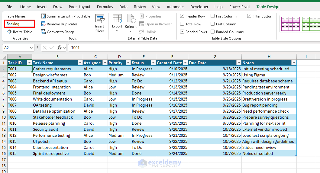
Name your table Backlog:
To DO Lookup:
Update the other task board following this format.
Regards,
ExcelDemy
Hello Chioma Laszczewska,
You are most welcome. Thanks for your feedback. Glad to hear that our tutorial was helpful to you.
Keep exploring Excel with ExcelDemy!
Regards,
ExcelDemy
Hello Ron Grehl,
The issue is with how SUMIF works. SUMIF only supports ONE condition, but your formula is trying to apply two conditions (>0 and =U), which is why Excel shows “too many arguments”.
To fix this, you should use SUMIFS instead.
Here’s the correct formula:
=SUMIFS(EG6:GN6, EG6:GN6, “>0”, EG7:GN7, “U”)
EG6:GN6 → values to sum
EG6:GN6, “>0” → only include values greater than 0
EG7:GN7, “U” → only include cells where row 7 has “U”
That should work perfectly.
Regards,
ExcelDemy
Hello A,
Thanks for your feedback. Glad to hear you liked our explanation.
Keep exploring Excel with ExcelDemy!
Regards,
ExcelDemy
Hello Ashish,
Thank you for sharing the detailed code and requirements—this is a very solid setup already. I’ve reviewed your logic and below are the key improvements and fixes to make it work exactly as expected.
Key Fixes & Enhancements
• 1. Fix alternate day condition (currently broken)
Replace this line:
If Day(todayDate) Mod 2 0 Then Exit Sub
With:
If Day(todayDate) Mod 2 0 Then Exit Sub
• 2. Fix date range condition (syntax issue)
Replace:
If todayDate >= startDate And todayDate endDate
With:
If todayDate >= startDate And todayDate <= endDate Then
• 3. Invoice Month logic (previous month required)
Replace:
ws.Cells(i, 6).Value = Format(Date, “mmmm yyyy”)
With:
ws.Cells(i, 6).Value = Format(DateAdd(“m”, -1, Date), “mmm yy”)
(This ensures April shows March, as required)
• 4. Define missing variable (important)
Add this before using it:
Dim isOverdue As Boolean
• 5. Correct overdue condition (after 20th)
Replace your overdue logic with:
If todayDate > endDate And invoicingStatus “raised” Then
sendMail = True
isOverdue = True
End If
• 6. Fix status update logic (Requirement 4 & 9)
Replace with:
If invoicingStatus = “raised” Then
ws.Cells(i, 14).Value = “Completed”
ElseIf isOverdue = True Then
ws.Cells(i, 14).Value = “Overdue”
Else
ws.Cells(i, 14).Value = “Pending”
End If
(This ensures email + status update happens correctly)
• 7. Ensure email still sends when status = raised (your issue)
Remove or adjust this line:
If lastSentStatus = “completed” Then GoTo NextRow
Replace with:
If lastSentStatus = “completed” And invoicingStatus = “raised” Then GoTo NextRow
(This allows first-time “raised” emails to send)
• 8. Add overdue message (Requirement 8)
Keep this (just improve formatting):
If isOverdue = True Then
overdueMsg = “This invoice is OVERDUE. Immediate action required”
End If
• 9. Improve email formatting (important)
Replace your email body with:
emailBody = “Dear Team,” & _
“Please find invoice details below:” & _
“Client Name: ” & ws.Cells(i, 1).Value & “” & _
“Project Name: ” & ws.Cells(i, 2).Value & “” & _
“PO No: ” & ws.Cells(i, 3).Value & “” & _
“Invoice Month: ” & ws.Cells(i, 6).Value & “” & _
“Status: ” & ws.Cells(i, 11).Value & “” & _
remarksText & “” & overdueMsg & _
“Regards,Automation System”
• 10. Remarks only for pending (already correct, just refine)
If invoicingStatus = “pending” Then
remarksText = “Remarks: ” & ws.Cells(i, 12).Value & “”
Else
remarksText = “”
End If
Regards,
ExcelDemy
Hello Diane,
Thank you for your detailed feedback and for going through the methods so carefully. The results you’re seeing are actually consistent in value, but they are presented in different formats, which can understandably cause confusion. Some methods (like TEXT and formatting-based ones) return the result as hours and minutes, while others (such as CONVERT and division/QUOTIENT approaches) return decimal hours.
For example:
• 3627.51 minutes ÷ 60 = 60.46 hours (decimal format)
• The same value expressed differently = 60 hours and ~27.5 minutes
So the difference isn’t in the calculation, but in how the result is displayed.
That said, you make a fair point that the article could present these outputs more consistently or clarify the distinction more explicitly. We’ll take that into account to improve clarity for readers.
Regards,
ExcelDemy
Hello Carol,
Thanks for your feedback! It should work in Microsoft Excel as well. Sometimes the steps or options may appear slightly different depending on your version or update. Please make sure you’re following the correct method for protecting the workbook structure, and feel free to share where you’re getting stuck—we’d be happy to help!
Regards,
ExcelDemy
Hello Alhassan Yusuf,
Please check your email inbox or spam folder. After subscribing the cheat list is automatically sent to your email address. Ensure you subscribed with valid email address.
We can’t send the file directly, please follow the download process.
Go to the Download Excel Formulas Cheat Sheet PDF & Excel Files section of this post and enter your valid email address.
Then check your inbox/spam folder to get the Excel file.
Regards,
ExcelDemy
Hello Ashish,
Thank you for your detailed follow-up and for sharing both the automation logic and the updated field list. This is shaping up to be a very well-structured solution.
Regarding your alert logic, your approach is absolutely practical and can be implemented with VBA:
• Alert duration (4th to 20th): You can control this using a date condition so emails are triggered only within this window.
• Alternate day alerts: The best approach is to track a “Last Reminder Sent Date” and send the next alert only if 2 days have passed. This is more reliable than using even/odd logic.
• Overdue alerts after the 20th: You can automatically mark pending invoices as “Overdue” and continue reminders until the status is updated to Completed.
Coming to your updated fields, your list already looks very good and covers most requirements. You may enhance it further with:
• Invoice Due Date – helps identify delays clearly
• Invoice Number – useful for tracking/reference
• Invoice Amount – helpful for reporting
• Last Reminder Sent Date – for automation control
• Email Status (Sent/Not Sent)
• Overdue Flag (Yes/No)
To make the file more user-friendly, you can also consider:
• Using dropdown lists for Invoicing Status and Reason for Delay
• Applying conditional formatting (e.g., highlight overdue items)
• Creating a simple dashboard for tracking (Pending vs Completed vs Overdue)
• Adding a manual trigger button for flexibility
Overall, your design is already very well thought out. With these enhancements, your automation will be even more efficient and user-friendly.
Regards,
ExcelDemy
Hello Ravi Kumar Sharma,
You are most welcome. Glad to hear that our article saved your years of data.
Keep exploring Excel with ExcelDemy!
Regards,
ExcelDemy
Hello Greg Lovern,
Thanks for your detailed and insightful feedback, we really appreciate you taking the time to clarify these points.
You’re absolutely right that VBA has long been supported on Excel for Mac, with the notable exception of Excel 2008, and that modern 64-bit versions continue to support it. Our intention in that line was to highlight practical limitations across platforms, especially that VBA doesn’t run in Excel for Web and may have reduced or inconsistent support in some macOS environments compared to Windows. We’ll look into refining that wording for better accuracy.
Regarding the VBA editor, thank you for pointing out the autocomplete feature, it’s true that it has existed for quite some time. Our comment was more about the lack of more advanced, modern IDE capabilities compared to environments used for JavaScript, but we agree this could have been better phrased.
On the syntax comparison, that’s a fair perspective as well—both VBA and JavaScript are relatively accessible, especially for beginners, and preference often depends on prior exposure.
We also appreciate your expectation about the article’s focus. Expanding more on the practical differences in automation capabilities between VBA and Google Apps Script is a great suggestion, and we’ll consider improving the content in that direction.
Thanks again for helping us improve!
Regards,
ExcelDemy
Walaikumassalam Miru,
Welcome to ExcelDemy! Yes if you go through all the practice and data entry practice pdf, you will be able to handle such issues easily.
To learn more about Excel, you can go though the Learn Excel guide.
Regards,
ExcelDemy
Hello User,
If you only need a simple confirmation without adding the file itself, then no—Excel doesn’t require attaching a PDF. However, if you want the PDF to be accessible directly from the workbook (for example as a reference document or report), attaching or embedding it using Insert → Object → Create from File is the recommended approach.
Let us know if you want the PDF to open with a click or just link to it—we can guide you further.
Regards,
ExcelDemy
Hello Timmy C.
It sounds like Excel may still be recognizing something far to the right of your visible data, which can affect how the horizontal scroll bar behaves. Even if your actual data ends at column Z, hidden objects, formatting, comments, or other elements can extend the used range of the worksheet.
You can try a few things to fix it:
1. Check for objects or formatting to the right
Press Ctrl + End to see where Excel thinks the last used cell is.
If it jumps somewhere far to the right (like column CXX or beyond), Excel is still detecting content there.
2. Clear unused columns
Select the first empty column after your real data (AA or AB, depending on your sheet).
Press Ctrl + Shift + Right Arrow to select all columns to the end.
Right-click and choose Delete (not just Clear Contents).
3. Save and reopen the workbook
After deleting the extra columns, save the file, close Excel, and reopen it. This resets the worksheet’s used range in many cases.
4. Check for hidden objects
Go to Home → Find & Select → Go To Special → Objects to see if any shapes, comments, or notes are placed far to the right.
Regarding Notes vs. Comments, they normally shouldn’t extend the scroll range by themselves, but if a note or object was accidentally placed far off to the right, Excel might treat that area as part of the used sheet, which can lead to scroll bar issues like the one you described.
If the problem still occurs specifically when column AE is hidden, it may indicate that AE contains some formatting or an object tied to that column. Clearing or deleting columns beyond your actual data usually resolves this.
Regards,
ExcelDemy
Hello Victor,
Good day! Have a nice day too. Yes, you can create a monthly report of daily sales in Excel. First, store your daily sales data in a table with columns like Date, Product/Item, Quantity, and Sales Amount. Then you can summarize the data monthly using formulas or PivotTables.
These ExcelDemy guides may help you step-by-step:
• How to Make a Sales Report in Excel
• How to Create Daily Sales Report in Excel
• Excel Cash Flow Template (useful for financial tracking and reporting)
You can follow these examples to organize your daily data and automatically generate monthly summaries.
Regards,
ExcelDemy
Hello Francis Vosena,
Thank you for your question. In Excel, column widths are applied to the entire column, so it’s not possible to set different column sizes for different rows within the same column. If you need more space in specific rows, you can try alternatives such as merging adjacent cells, using Wrap Text, or adjusting row height to better fit the content. Another option is to split the data into separate columns or sections where different column widths can be applied.
Regards,
ExcelDemy
Hello Mike G,
This usually happens when Excel doesn’t recognize your intended X-axis values or when the chart type is set to use default row numbers.
You can fix it by manually assigning the correct X-axis range:
1. Click on the chart.
2. Go to Chart Design → Select Data.
3. Under Horizontal (Category) Axis Labels, click Edit.
4. Select the cells that contain your actual column values for the X-axis.
5. Click OK.
Also make sure the X-axis data is formatted as numbers (not text). If Excel reads them as text, it may default to row numbers instead.
Regards,
ExcelDemy
Hello Emre Çakır,
The “UTMNorthing” error usually occurs due to an issue with the Latitude value or the cell reference used in the formula. Since UTMEasting and UTMZone are working correctly, the problem is most likely related to the input format or reference used for the latitude.
Please check the following:
1. Make sure the Latitude and Longitude values are formatted as Number, not Text.
2. Verify that the cell references in the UTMNorthing formula point to the correct cells.
3. Check if there is any issue with the decimal separator (dot vs comma) depending on your regional settings.
4. In some regional settings, you may need to use semicolon (;) instead of comma (,) in the formula.
After checking these points, the issue is usually resolved. If the problem persists, please share a sample Latitude and Longitude value you are using so I can help you troubleshoot further.
Regards,
ExcelDemy
Hello Ashish
Yes, this can be done with a customized Excel template and updated VBA code. The previous sample was a basic version, but for your case the sheet should be structured row-wise so each PO is treated separately and emails can go automatically to all recipients mentioned in that row. Use the following VBA code with a sheet structured like this:
A = Client Name
B = PO No
C = PO End Date
D = Project Manager Name
E = To Email
F = CC Email
G = Additional Email(s)
H = Remarks / Status
I = Last Sent On
J = Last Sent Status
If you want it to run when the workbook opens, paste this into ThisWorkbook:
A few important notes:
This code sends one email per PO row
If the same manager has multiple POs, they will get multiple separate emails
If the date is extended, the next reminders will follow the new date
If the row is deleted, reminders stop automatically
Column I prevents sending the same reminder multiple times on the same day
For fully automatic sending at a fixed time, Excel must still be launched by Windows Task Scheduler.
Regards,
ExcelDemy
Hello Sanny,
If you want to insert a picture in a document that uses outlines, you can still do it easily. Place your cursor where you want the image to appear, then go to Insert → Pictures and choose the image from your device. The picture will be inserted at that position.
Keep in mind that pictures don’t become part of the outline structure because outlines are based on heading levels (Heading 1, Heading 2, etc.). If you want the picture to stay organized within a section, simply insert it under the relevant heading. This way, when you collapse or expand sections using the outline, the picture will remain within that section.
You can also add a caption to the picture (References → Insert Caption) to make it easier to identify and reference in the document.
Regards,
ExcelDemy
Hello Ashish,
Thank you for your detailed feedback. I’m glad you found the automation helpful. Here’s an updated VBA version you can use as a replacement for the basic code. It covers your requested changes.
Assumed sheet structure
This code assumes your sheet looks like this:
A = Person Name
B = Email
C = Item / Document / Task Name
D = Deadline
E = Department
F = Remarks
You can change the column letters inside the code if needed.
VBA Code:
Regards,
ExcelDemy
Hello Kenneth,
Please check your email inbox or spam folder. After subscribing the cheat list is automatically sent to your email address. Ensure you subscribed with valid email address.
We can’t send the file directly, please follow the download process.
Go to the Download Excel Formulas Cheat Sheet PDF & Excel Files section of this post and enter your valid email address.
Then check your inbox/spam folder to get the Excel file.
Regards,
ExcelDemy
Hello Stephanie,
You are most welcome. Thanks for your feedback and appreciation. Glad to hear it was helpful.
Keep exploring Excel with ExcelDemy!
Regards,
ExcelDemy
Hello Peter,
You are most welcome. Thanks for your feedback and appreciation. Glad to hear our suggestion was helpful.
Keep exploring Excel with ExcelDemy!
Regards,
ExcelDemy
Hello Raisa,
The Error 13 – Type mismatch almost always happens in this kind of code when:
1. One or more cells in your search ranges (B13:M99999 on sheets IN, IS, LU, PA) contain non-string values like numbers, dates, errors (#N/A, #VALUE!, #DIV/0!), booleans, or empty cells treated incorrectly.
2. The PartialMatch function does Mid(Value2, i, Len(Value1)) or LCase(Value2) — but if Value2 is not a string (e.g. it’s a number or error value), VBA throws Type mismatch.
Quick fixes for the error:
Force Value2 to be treated as a string — this is the simplest and usually solves 90% of these cases.Change this line inside the loop:
Value2 = Rng.Cells(i, j).Value
to:
Value2 = CStr(Rng.Cells(i, j).Value & “”)
CStr() converts numbers/dates to string.
& “” turns errors/nulls into empty string instead of crashing.
Skip error values completely (even safer):
Replace the Value2 line with:
If IsError(Rng.Cells(i, j).Value) Then GoTo NextCell
Value2 = CStr(Rng.Cells(i, j).Value)
And add a label just before Next j:
vbaNextCell:
Next
Update your PartialMatch function to be more robust:
Function PartialMatch(Value1 As Variant, Value2 As Variant, Case_Sensitive As Boolean) As Boolean
Dim s1 As String, s2 As String
If IsEmpty(Value1) Or IsEmpty(Value2) Then
PartialMatch = False
Exit Function
End If
‘ Convert to strings safely
s1 = CStr(Value1)
s2 = CStr(Value2 & “”) ‘ & “” prevents error values from crashing
If Not Case_Sensitive Then
s1 = LCase(s1)
s2 = LCase(s2)
End If
PartialMatch = (InStr(1, s2, s1, vbBinaryCompare) > 0) ‘ much faster & cleaner than Mid loop!
End Function
Replace Mid loop with InStr — it’s built-in, faster, and does exactly the same substring search. Handles empty cells gracefully.
Regards,
ExcelDemy
Hello Frank,
It can definitely feel that way sometimes! But small tweaks—like changing the default date format—can save you a lot of time in the long run. If you follow the steps in the article, you only need to set it once and Excel will use your preferred format automatically.
If you run into any issues while applying the method, feel free to share the details and we’ll be happy to help.
Regards,
ExcelDemy
Hello Ichal,
You are most welcome. Thanks for your appreciation. Keep exploring Excel with Exceldemy!
Regards,
ExcelDemy
Hello Ichal,
You are most welcome. Thanks for your appreciation. Keep exploring Excel with Exceldemy!
Regards,
ExcelDemy
Hello Amy,
You are most welcome. Thanks for your feedback and appreciation. Glad to hear that your problem is solved.
Keep learning Excel with ExcelDemy!
Regards,
ExcelDemy
Hello Low,
Thank you for your comment! If a workbook is protected with a password (especially with structure protection or encryption), Excel will block access to features like adding or running macros until the correct password is entered. That’s why the VBA method only works if you can still open the workbook or if the structure isn’t fully locked.
In cases where the file is fully encrypted and you don’t know the password, Excel won’t allow any modifications, including inserting macros.
Regards,
ExcelDemy
Hello Frede,
Thank you for pointing that out. The wording in that paragraph was unclear and made it seem like two things needed to be selected at the same time. We’ve updated the article to clarify that the steps should be done sequentially (first select the range, next copy it, then select the destination cell).
We really appreciate your careful reading and helpful feedback!
Regards,
ExcelDemy
Hello Jenna,
When you enter 0430 in a cell formatted as time, Excel treats it as a serial number instead of 04:30, which is why it converts it to an unexpected date/time value. Custom formatting alone doesn’t change how Excel interprets the raw input.
Formatting the column as Text is definitely one practical solution if you just want to store HHMM exactly as typed. However, if you want Excel to recognize it as a real time value (so you can calculate with it), you can also use a formula-based approach. For example, if A1 contains 0430, you can use:
=TIME(LEFT(A1,2),RIGHT(A1,2),0)
This converts HHMM into a proper Excel time (04:30) that works in calculations.
Excel’s behavior can be frustrating at times, but once we understand how it stores dates and times as serial numbers, it becomes easier to control the outcome. Thanks again for pointing this out—it’s a very practical concern for many users.
Regards,
ExcelDemy
Hello Vicki,
Thank you so much for your thoughtful feedback and for choosing ExcelDemy for your learning journey! You’re absolutely right, understanding what the functions actually do makes a big difference. Here’s a quick explanation:
TRIM: Removes extra spaces from text, leaving only single spaces between words (and removes leading/trailing spaces).
CLEAN: Removes non-printable characters (like line breaks or hidden characters that often come from copied data).
SUBSTITUTE / SPACE: SPACE(n) adds a specified number of spaces, and SUBSTITUTE is often used to replace specific characters (including unwanted spaces).
We truly appreciate your suggestion, adding clearer explanations of each function’s purpose would definitely make the page even more helpful. Thanks again for sharing your experience!
Regards,
ExcelDemy
Hello Erkan,
Thanks for your appreciation and feedback. Glad to hear it was helpful. Keep exploring Excel with ExcelDemy!
Takdiriniz ve geri bildiriminiz için teşekkürler. Faydalı olduğunu duymak beni mutlu etti. ExcelDemy ile Excel’i keşfetmeye devam edin!
Regards,
ExcelDemy
Hello Ronald Brown,
Yes, it’s possible, but TEXTJOIN alone can’t sort. You need to SORT the names first, then wrap them in TEXTJOIN.
Assuming your data is in:
A2:D2
A2 = LastFirst
B2 = Roommate#1
C2 = Roommate#2
D2 = Roommate#3
Use this formula (Excel 365 / Excel 2021):
=TEXTJOIN(“, “, TRUE, SORT(A2:D2))
Why this works:
SORT(A2:D2) → sorts all four names alphabetically
TEXTJOIN(“, “, TRUE, …) → joins them into one cell, separated by commas
Since the names are already written as LastName FirstName, sorting automatically:
Sorts by Last Name
Then by First Name when last names are the same
Regards,
ExcelDemy
Hello Love,
You are most welcome. Thanks for your feedback and appreciation. Glad to hear that our SUMIFS formula helped you to solve problem.
Keep exploring Excel with ExcelDemy!
Regards,
ExcelDemy
Hello Syed,
Thanks for your feedback and appreciation. Glad to hear that you liked our tutorial.
Keep exploring Excel with ExcelDemy!
Regards,
ExcelDemy
Hello Jim,
That’s actually a very practical workaround. Yes, using Find & Replace with double spaces → single space works, especially when you just need a quick cleanup without formulas.
However, as you mentioned, you may need to click Replace All multiple times until Excel removes all consecutive spaces. This happens because Excel replaces only two spaces at a time — so if there are 4 or 5 spaces, it reduces them step by step.
For a cleaner and more reliable method, you can use:
=TRIM(A1)
The TRIM function automatically:
Removes extra spaces between words
Keeps only single spaces
Removes leading and trailing spaces
If your data also contains non-breaking spaces (often copied from websites), you can use:
If TRIM doesn’t work, try combining TRIM with SUBSTITUTE to replace non-breaking spaces with regular spaces first.
This handles hidden spaces that TRIM alone doesn’t remove.
So your method works, but formulas can save time when working with large datasets.
Regards,
ExcelDemy
Hello Eichelle Myka,
To check your grades correctly in Excel, first make sure all your marks are entered properly as numbers (not text). Even a small typing error can affect the result.
Then:
Calculate the Total using:
=SUM(B2:F2)
Calculate the Average using:
=AVERAGE(B2:F2)
Apply the grading formula based on your scale. For example:
=IF(G2>=90,”A”,IF(G2>=80,”B”,IF(G2>=70,”C”,IF(G2>=60,”D”,”F”))))
Also check the following:
1. Your grading scale is correct.
2. The formula references the correct cells.
3. You are not missing any subjects in the calculation.
4. If the grades are weighted, confirm that the weights are applied properly.
Regards,
ExcelDemy
Hello Nancy,
You can do this with a simple lookup table and a formula.
Create a small table (anywhere) like:
D2:D = Driver Name
E2:E = Percent (enter as 20%, 15%, 0%, etc.)
Then in A3 use either of these:
XLOOKUP (recommended):
=A2*XLOOKUP(A1,$D$2:$D$100,$E$2:$E$100,0)
Or VLOOKUP:
=A2*VLOOKUP(A1,$D$2:$E$100,2,FALSE)
So if A1 = Dan and his rate is 20%, A3 returns 20% of A2. If A1 = Bob and his rate is 15%, it returns 15% of A2. If the name isn’t found, it returns 0 (you can change that behavior if you want).
Regards,
ExcelDemy
Hello Amy,
Yes, it’s possible to hide non-zero data labels and show only the zero values in an Excel chart. You can do it using a helper column.
1. Suppose your original values are in B2:B10.
2. In a new column (say C2), enter this formula:
=IF(B2=0,B2,””)
3. Fill the formula down.
4. Select your chart → click on Data Labels → choose Format Data Labels.
5. Under Label Options, check Value From Cells and select the helper column (C2:C10).
6.Uncheck the default Value option if needed.
Now only the zero values will appear as labels, and all non-zero labels will remain hidden.
Regards,
ExcelDemy
Hello Uwibambe Marie Gorethi,
You can explore our this Calculation with Excel Formulas category to get more exercise for practice. Hopefully you will understand better after completing all the tasks.
Regards,
ExcelDemy
Hello Duke,
You are most welcome. Thanks for your feedback and appreciation.
Keep exploring Excel with ExcelDemy!
Regards,
ExcelDemy
Hello Core,
Thanks for the clear question. Yes, the schedule does factor in the reduced principal balance when recalculating payments after a rate change.
In this setup, interest is always calculated from the current outstanding balance (the remaining principal after all payments made up to that point), not from the original loan amount. So if the interest rate changes after the first 12 months, the “new repayment” (or revised payment amount, depending on how you set it up) is based on the balance at month 12, then it continues amortizing from there. It does not restart from the initial principal.
If you are updating the rate in the input cell(s), just make sure the formula for interest is referencing the previous period’s ending balance (or current balance row), and the payment recalculation (e.g., PMT) is using that remaining balance as the present value. That’s the key “smart” link that ensures everything stays accurate after the rate update.
Best regards,
ExcelDemy
Hello Sandro,
Good afternoon! You’re very close already, the main issue is how the date is written back to the TextBox/cell, not how it’s displayed inside the calendar.
Right now, this line is the key problem:
TargetControl.Value = CDate(Me.TextBox1)
CDate converts the text back to a date serial, and Excel then formats it using US regional settings, even if the string looks Italian.
Correct way to force Italian format (dd/mm/yyyy)
You should write the formatted text, not reconvert it with CDate.
Option 1: Force format for a TextBox (recommended)
Replace this part:
TargetControl.Value = CDate(Me.TextBox1)
with:
TargetControl.Value = Format(Me.TextBox1.Value, “dd/mm/yyyy”)
This guarantees the TextBox always shows Italian format, regardless of Excel language.
Option 2: If the target is a worksheet cell
If TargetControl is a Range, force the cell’s number format explicitly:
With TargetControl
.NumberFormat = “dd/mm/yyyy”
.Value = VBA.CDate(Me.TextBox1.Value)
End With
This keeps the value as a real date and displays it in Italian format.
Format(…, “dd/mm/yyyy”) controls display
NumberFormat = “dd/mm/yyyy” overrides Excel’s regional defaults
Avoiding CDate on TextBoxes prevents Excel from re-interpreting the date as US (mm/dd/yyyy)
Regards,
ExcelDemy
Hello Demetri,
Please check your email inbox or spam folder. After subscribing, the file is automatically sent to your email address. Ensure you subscribed with valid email address.
Or you can follow the steps again,
go to the Download section of this post and enter your email address.
Then check your inbox/spam folder to get the Excel file.
Regards
ExcelDemy
Hello Stephanie Powell,
This template can be adapted for interest-only payments for an initial period. You’d handle it by calculating interest only (balance × rate) for those months and keeping the principal unchanged. After the interest-only period ends, you switch the formula back to the normal amortization calculation so payments include both principal + interest based on the remaining balance and term.
Regards,
ExcelDemy
Hello KK,
The article currently demonstrates Delta E using the CIE76 method only.
CIEDE2000 (Delta E 2000) is more complex and requires several intermediate calculations.
However, CIEDE2000 can be implemented in Excel by adding extra columns for the intermediate steps or by using a single Excel 365 formula.
Regards,
ExcelDemy
Hello Xen,
You are most welcome. Thanks for your feedback and appreciation.
Keep exploring Excel with ExcelDemy!
Regards,
ExcelDemy
Hello Y.Narasimha Rao,
You are most welcome. Thanks for your appreciation.
Keep learning Excel with ExcelDemy!
Regards,
ExcelDemy
Hello Brian,
You’re right to think about the actual number of days—that’s the key point here. Excel’s FV function can handle a 9-month period with daily compounding, but it does not work well if you simply enter 9/12 or 0.75 for years when compounding daily.
Here’s how it should be handled conceptually in Excel:
FV does not need start and end dates directly, but you must convert the 9-month period into the correct number of days, then use that as nper.
For daily compounding:
rate = annual_rate / 365
nper = actual number of days between the start and end dates
For example:
Start date: Jan 1
End date: Sep 30
Days = DATEDIF(start_date, end_date, “d”)
Then the formula structure becomes:
=FV(annual_rate/365, number_of_days, 0, -present_value)
This avoids the problem you noticed with 9/12 or 0.75, which only makes sense for annual or monthly compounding, not daily compounding.
And you’re absolutely correct that different 9-month ranges will produce different results, because the number of days varies (leap years, month lengths, etc.). That’s why using actual dates (or actual day counts) is the accurate approach.
Great observation, this is exactly the kind of nuance that trips people up with financial functions.
Regards,
ExcelDemy
Hello Rebecca Tracy,
Thanks for your appreciation. The sheet is protected but it is not password protected.
You just need to go to the Review tab >> select Unprotect Sheet.
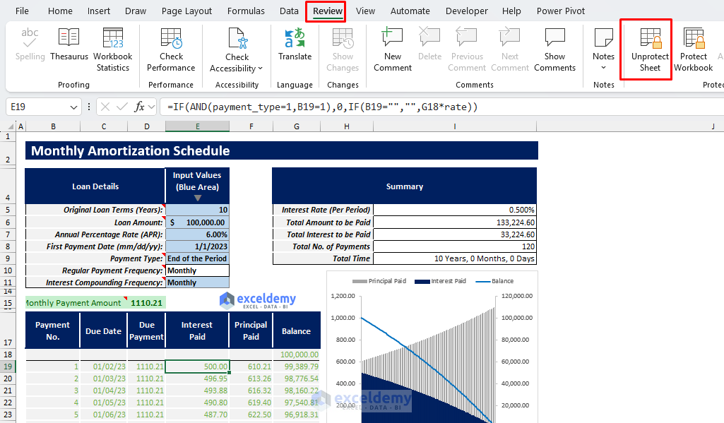
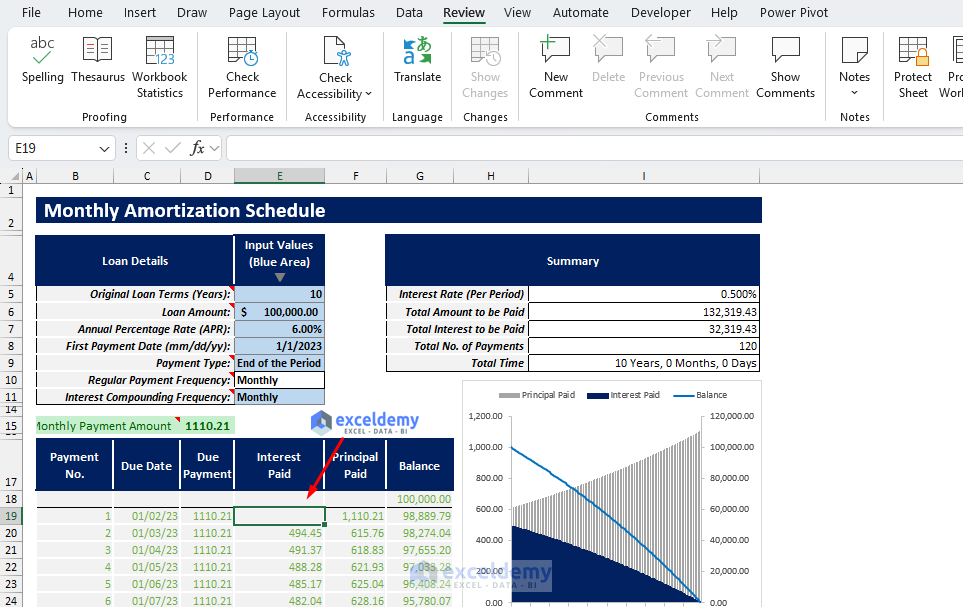
It will remove the sheet protection.
Now you can add, update or delete or alter the sheet.
If the issue still persist, you can download the following file, I removed the sheet protection.
Excel Monthly Amortization Schedule.xlsx
Regards,
ExcelDemy
Hello Harry,
You are most welcome. Thanks for your feedback and appreciation.
Keep exploring Excel with ExcelDemy!
Regards,
ExcelDemy
Hello Marcel,
If you forget the password of an Excel file, Excel itself doesn’t provide a built-in way to recover or remove it. The available options are:
1. Check if the file owner or creator can resend the file or share the password
2. Restore an earlier unprotected version from backup (OneDrive, Google Drive, File History, etc.)
3. If it’s a sheet/workbook structure password (not file-open password), VBA-based recovery methods may work
4. For file-open passwords, you’ll need the original password or a professional recovery tool
Regards,
ExcelDemy
Hello Marcel Williams,
Thanks for your feedback and appreciation. Glad to hear you liked our content.
Keep exploring Excel with ExcelDemy!
Regards,
ExcelDemy
Hello Usman,
Thanks for your feedback and appreciation. Glad to hear that you liked our tutorial.
We attached the sample file in our article for better practice.
Regards,
ExcelDemy
Hello Hasina Khan,
That’s great to hear! If you’re just starting with Excel, this article is designed specifically for beginners and explains everything in a clear, step-by-step way—from understanding the Excel interface to entering data, using basic formulas, and creating simple tables and charts. It helps you build a strong foundation without feeling overwhelmed.
In addition, you can also check out this complete Excel learning hub:
Learn Excel
This page is very useful because it organizes Excel tutorials by skill level (Beginner, Intermediate, and Advanced). You can start with essential topics like formatting cells, basic functions (SUM, AVERAGE, IF), and data entry, then gradually move on to more advanced features such as lookup functions, PivotTables, charts, and automation.
Using both resources together is a great approach: start with the beginner article to understand the basics, then use the learning hub to practice and expand your skills step by step. If you get stuck or want to learn a specific feature, feel free to ask.
Happy learning!
Regards,
ExcelDemy
Hello Bill,
The #VALUE! error usually happens when Excel can’t recognize the date text as a valid date.
Please double-check that the date is stored as text (not already a date), the text format matches your system’s regional date settings, and there are no extra spaces in the cell.
You can also try using TRIM() or adjusting the date format (for example, MM/DD/YYYY vs DD/MM/YYYY). Let us know the exact date value you’re using, and we’ll be happy to help further.
Regards,
ExcelDemy
Hello Anthony,
Hi, thanks for checking this. The file is working as intended. When Remaining Years is less than the original loan term, the calculator applies the recurring extra payment only to the remaining amortization period and calculates interest savings relative to the remaining balance, not the original 30-year schedule.
Because interest that has already accrued cannot be saved, the impact of a smaller extra amount (like 50) may appear limited when fewer years remain, even though the extra payment logic is being applied correctly.
So this behavior is expected and not a formula error in the Excel file.
Regards,
ExcelDemy
Hello Nicolas G Pepin,
Thanks for sharing this project. It’s interesting to see an Excel-native approach to introducing ML concepts without external tools. This could be useful for users who want to explore ML ideas directly inside Excel.
Regards,
ExcelDemy
Hello Tom,
Hi, this usually happens when Power Query can’t detect your Google Sheet as a structured HTML table. A few things to check:
1. Make sure the Google Sheet is published correctly:
Go to File → Share → Publish to web and publish the entire sheet (or the specific tab) as a web page. Then copy the generated URL and use that one in Power Query (not the normal share link).
2. Ensure the data is in a proper table layout:
No completely blank rows at the top
Headers must be in the first row
Avoid merged cells; Power Query relies on clean HTML tables; otherwise it collapses everything into one column.
3. If only one column loads:
That means Power Query is reading the page as raw HTML, not a data table. In that case:
Select HTML Tables → Table 1
Click Transform Data
Use Split Column → By Delimiter or Use First Row as Headers if needed
4. Alternative (more reliable) option:
Export the Google Sheet as CSV (File → Share → Publish → CSV) and connect to that CSV URL instead. This avoids the HTML table limitation and loads all columns correctly.
Once the sheet is properly published and structured, Power Query should detect all columns normally.
Regards,
ExcelDemy
Hello Ogirima,
You can download the Excel and PDF files free of cost just by entering your valid email address in the download section. To get the files go to the “Download Excel Formulas Cheat Sheet PDF & Excel Files” section of this post and enter your email address.
Then check your inbox/spam folder to get the Excel file.
Best Regards
ExcelDemy
Hello Dear,
You’re right that the example is simple linear regression—but linear regression is also one of the most common machine learning (supervised learning) methods. In the article, it’s used as a beginner-friendly ML starting point.
If you’d like, we can add a quick note and show a more “classic ML” Excel example too (e.g., classification with logistic regression or a basic decision-tree-style model).
Regards,
ExcelDemy
Hello Kelly,
Thanks for trying it out. Yes, this is a common situation. Even if the flow test says “successful”, the email won’t appear unless the trigger condition is actually met.
A few things to double-check:
1. Make sure the condition (e.g., cell value change / threshold) is truly met in Excel after the flow is turned on.
2. Confirm the email action is correctly configured (recipient address, subject, body).
3. Check the Run History in Power Automate and open the run details to see if the email step was skipped.
3. If you’re using Excel Online, ensure the file is saved in OneDrive(Business) or SharePoint, not locally.
4. Try updating the data again after enabling the flow. That usually fixes it. Hope this helps!
Regards,
ExcelDemy
Hello Usman,
Here is our Excel file for practice: How to Build Nested IF Statements in a Single Cell
Practice and let us know your feedback and experience.
Regards,
ExcelDemy
Hello king,
Thanks for your feedback and appreciation. Glad to hear that you liked our article.
Keep exploring Excel with ExcelDemy!
Regards,
ExcelDemy
Hello Godfrey,
Thanks for your comment! Sure—please let me know what specific part you’d like help with, and I’ll be happy to assist you step by step.
Regards,
ExcelDemy
Hello Gayla,
You are most welcome. Thanks for your feedback. Glad to hear that you really liked our instructions and explanations.
Keep exploring Excel with ExcelDemy!
Regards,
ExcelDemy
Hello Vaibhav,
Thank you for your question. For complicated calculations, Excel’s built-in functions are usually more reliable and easier to maintain than doing everything in VBA. Depending on the type of analysis, you can combine dynamic array functions (like FILTER, UNIQUE, SORT), lookup functions (XLOOKUP, INDEX + MATCH), and aggregation functions (SUMIFS, COUNTIFS, AVERAGEIFS).
If the logic is very complex, breaking calculations into helper columns using these functions often makes the model clearer and reduces VBA complexity. VBA can then focus mainly on automating the report generation and exporting results to Word, rather than performing the calculations themselves.
Regards,
ExcelDemy
Hello Mohammad Afzal,
Thank you for your feedback! Yes, survey data analysis with Pivot Tables can feel intense at first, but once the core concepts are clear, it becomes much more manageable and very powerful for real-world analysis.
Regards,
ExcelDemy
Hello Va,
This usually happens when a formula is referencing an external workbook (for example, a cell or sheet that was copied from another file). When Excel can’t find that source, it prompts you with a File Open dialog.
Here’s what you can check:
1. Make sure all formulas in the Summary sheet refer only to sheets within the same workbook.
2. If you copied any formulas from another Excel file, re-enter them manually instead of pasting.
3. Check the formula bar for links like [WorkbookName.xlsx]SheetName! and remove those external references.
4. Also confirm that sheet names match exactly as shown in the tutorial.
Once all external links are removed, copying the cells should work without opening a file dialog.
Regards,
ExcelDemy
Hello Christof,
When a worksheet is protected, the “Clear Filter” button on the Data tab is disabled, even if Use AutoFilter is allowed during protection. Excel only permits clearing filters from the filter drop-down arrows, not from the ribbon, on protected sheets.
What you can do instead:
1. Clear filters using each column’s filter drop-down.
2. Temporarily unprotect the sheet, clear all filters from the ribbon, then protect it again.
3. Use a small VBA macro (with a button) to unprotect → clear filters → reprotect the sheet in one click.
So unfortunately, there is no native way to enable the ribbon’s “Clear Filter” button while the sheet remains protected—this is by design in Excel.
Regards,
ExcelDemy
Hello Jon Nelson,
Thanks for the detailed feedback, this is a very valid point. You’re right that many of the examples in the article assume a specific date order (like day–month–year), which can cause issues when your data is in year–month–day (YYYY-MM-DD) format or when formats are inconsistent.
A more robust approach that works regardless of the displayed order is to first make sure Excel is working with a true date value, and then extract the components using built-in date functions:
Year: =YEAR(A1)
Month: =MONTH(A1)
Day: =DAY(A1)
These functions are format-independent and will continue to work even if the date format changes unexpectedly in large datasets.
If some of your dates are stored as text (which often happens with imported files), you can first convert them using:
Go to the Data tab >> select Text to Columns, or
=DATEVALUE(A1) (when Excel can recognize the text date)
Once converted, YEAR(), MONTH(), and DAY() will handle both Y-M-D and D-M-Y formats reliably without relying on LEFT, MID, or RIGHT. Thanks again for pointing this out, it’s a great real-world scenario, especially when working with large and inconsistent data files.
Regards,
ExcelDemy
Hello Donna,
This isn’t a margins issue. What you’re seeing happens when Row and Column Headings are enabled for printing. Excel is including the A, B, C… and 1, 2, 3… labels on the printed page.
To fix it:
1. Go to the Page Layout tab.
2. In the Sheet Options group >> find Headings.
3. Uncheck the Print box under Headings.
Alternatively:
Press Ctrl + P >> click Page Setup >> go to the Sheet tab >> uncheck Row and column headings >> click OK.
After this, your worksheet will print without the row and column labels.
Regards,
ExcelDemy
Hello Sarveshkumar Gupta,
Thank you for downloading the file and for taking the time to describe the issue so clearly. You are correct in your observation. In the current version of the worksheet (last updated on 29-10-2023), extra irregular payments are applied to the Principal Paid calculation, which is why you see their effect in the schedule rows. However, the total number of payments is kept fixed at 360, so the model does not dynamically shorten the loan term when extra payments are made. Because of this design choice, the summary section and the “Time Saved” calculation do not automatically update based on irregular extra payments.
To fully support extra payments that reduce the loan duration, the schedule would need to:
1. Dynamically stop once the remaining balance reaches zero (instead of forcing 360 rows), and
2. Recalculate the summary metrics (total payments, interest paid, and time saved) based on the actual payoff period.
This would require a more advanced setup using either dynamic arrays (in Excel 365) or VBA to handle variable loan length cleanly. Regarding your request for accommodating 20 different interest rates, that is definitely possible, but it would require restructuring the interest-rate timeline and the underlying formulas so the model can switch rates seamlessly while also handling early payoff logic.
Thank you again for pointing this out. This feedback is very helpful, and the article/template will be reviewed for a future update to better address these advanced scenarios.
Regards,
ExcelDemy
Hello Fiona,
Thanks for your feedback and for trying out the tutorial! This error usually occurs when the slicer is filtering a non-contiguous date range (for example, selecting individual months or years instead of a continuous period). The SAMEPERIODLASTYEAR() function in Power Pivot requires a continuous, properly related Date table.
Please check the following points:
1. Make sure you are using a dedicated Calendar/Date table (not the date column directly from the sales table).
2. Ensure the Date table is marked as a Date Table in Power Pivot.
3. Confirm that the slicer is connected to the Date table, not the fact table.
4. When using the slicer, select a continuous range (e.g., a full year or consecutive months).
Once these conditions are met, the YOY Growth measure should work correctly with the slicer. Let us know if the issue persists!
Regards,
ExcelDemy
Hello,
Here is the practice file: 5 PivotTable Tricks to Unlock Deeper Insights in Your Data
By following my tutorial practice all the tricks to unlock deeper insights.
Regards,
ExcelDemy
Hello Sifatullah,
You are most welcome. Thanks for your feedback and appreciation. Glad to hear that our tutorial is helping you to understand the fundamental of Pivot Tables in Excel.
Keep exploring Excel with ExcelDemy!
Regards,
ExcelDemy
Hello April,
You are most welcome. Thanks for your appreciation.
Keep exploring Excel with ExcelDemy!
Regards,
ExcelDemy
Hello Drik,
Thank you very much for pointing this out and for your kind words. You’re absolutely right—this issue happens because the script is not handling special (non-ASCII) characters like ä, Ä, Ö, Ü correctly. By default, many encoding/decoding scripts assume ASCII or a limited character set, so those characters can get lost during decoding.
How to fix it:
The solution is to explicitly use UTF-8 encoding when converting or processing the text. UTF-8 fully supports German umlauts and other special characters.
For example, if the script uses VBA or a text-based encoding step, make sure:
1. The text is converted using UTF-8 (not ASCII).
2. Any StrConv, Chr, Asc, or byte-array conversion is replaced with a UTF-8–aware approach.
Once UTF-8 encoding is applied consistently in both the encoding and decoding steps, characters like ä, Ä, Ö, Ü will be preserved correctly.
Thanks again for reporting this, feedback like yours helps improve the solution for everyone. Glad to hear you liked it overall!
Regards,
ExcelDemy
Hello Sajid,
You can do this very easily by making a small adjustment after converting the number to words.
If you are using the VBA function from this article:
Simply append the word “ Only” at the end of the returned text.
Option 1: Using a formula (no VBA edit required)
If your formula is:
=NumberToWords(A1)
use:
=NumberToWords(A1) & ” Only”
This will display:
5000 → Five Thousand Only
Option 2: Editing the VBA function (permanent solution)
Inside the VBA function, add ” Only” to the final return line so every output automatically ends with Only.
Both approaches work—use the formula method if you want flexibility, or edit the VBA code if you want “Only” added by default for all results.
Regards,
ExcelDemy
Hello Randall Helweg,
You can do this by treating the same input cell in two different ways—once as text and once as a calculated value.
If your INPUT CELL (say A1) contains the text 13/15:
1. To display it as a fraction (text)
In your report table column, simply reference the cell directly:
=A1
Make sure the cell format is Text so Excel doesn’t try to calculate it.
2. To display it as a percentage in the next column
Convert the text into a calculation using a formula like:
=LEFT(A1,FIND(“/”,A1)-1)/MID(A1,FIND(“/”,A1)+1,LEN(A1))
Then format this cell as Percentage (%).
This way, you are:
1. Displaying the original fraction exactly as entered in one column
2. Showing the calculated FG percentage from the same input cell in the next column
No need to change how the user inputs the data—Excel can handle both views from the same cell.
Regards,
ExcelDemy
Hello Samina,
You are most welcome. Thanks for your feedback and appreciation. I’m really glad the datasets were helpful for getting started with BTEC Information Technology. If you need any specific type of dataset or help using them in Excel, feel free to ask.
Keep exploring Excel with ExcelDemy!
Regards,
ExcelDemy
Hello Frida,
You are most welcome. Thanks for your appreciation.
Keep exploring Excel with ExcelDemy!
Regards,
ExcelDemy
Hello Steve,
Method 1 is indeed based on Office Scripts in Excel for the web, which is why Power Automate shows the trigger as “Schedule and Office Script to run in Excel.” This method does not behave like a traditional instant “button trigger” and works only under specific conditions (Excel for the web, OneDrive/SharePoint storage, correct account and script setup).
If this approach doesn’t trigger the flow in your case, we recommend using Method 2 or Method 3 from the article, which are more reliable for triggering Power Automate or Power BI actions directly from Excel.
Thanks for pointing this out, it helps clarify this limitation for other readers as well.
Regards,
ExcelDemy
Hello Sir,
Thank you very much for your kind words. The full method for calculating area, existing ground level (EGL), OGL, and their elevation differences for road earthwork (cut & fill) is already explained step by step in the article, along with formulas and an example dataset.
For clarity, the basic idea is:
Calculate difference = OGL − EGL at each station
Compute area using the Average End Area method
Then calculate cut/fill volume = (Area₁ + Area₂) / 2 × distance
You can follow the same steps shown in the tutorial using your own survey readings, and it will give you accurate executed work quantities.
If you get stuck at any step, feel free to ask here.
Regards,
ExcelDemy
Hello Susan,
You are most welcome and thanks a lot for your feedback. Basic VBA usually focuses on splitting the data, so things like extra blank rows, column spacing, frozen top rows, and filters don’t always carry over by default.
The good news is that all of these can be preserved with a few small additions to the code (for example, copying row heights, column widths, applying FreezePanes, and re-enabling filters after the split). If you’d like, you can share which formatting is most important for your case, and the VBA can be adjusted accordingly.
Really glad to hear the article was still helpful. Many thanks for taking the time to comment!
Regards,
ExcelDemy
Hello Zaenal,
You can share your file in our ExcelDemy Forum. Please explain your problem with proper images and in detail.
We would be happy to help you.
Regards,
ExcelDemy
Hello Mohammad Afzal,
Thanks for your feedback and appreciation. Glad to hear that you found our tutorial good and helpful. Keep exploring Excel with ExcelDemy!
Regards,
ExcelDemy
Hello David,
You can do this by posting a link to the cell value, not by copying the formula itself. If you want the cell on Sheet2 to always reflect the result of Sheet1!C3, use a formula reference when posting it.
For example, in VBA:
Sheets(“Sheet2”).Range(“A3”).Formula = “=Sheet1!C3”
This way:
Sheet1!C3 can contain any formula (like =$A$1+$B$1)
Sheet2!A3 will always update automatically when the value of Sheet1!C3 changes
If you instead copy the formula itself, Excel will recalculate it locally on Sheet2, which is not what you want in this case. Linking to the cell ensures Sheet2 stays synchronized with Sheet1.
Regards,
ExcelDemy
Hello Ashu Rani,
Yes, you can absolutely do data entry in Excel. Just type the information into the rows and columns and press Ctrl + S to save. Our page have articles to guide you step-by-step using the practice sheet from the article—telling you exactly what to enter in each column.
Regards,
ExcelDemy
Hello Snootch,
You are most welcome. Thanks for your appreciation and feedback. Glad to hear that our page is helful to you.
Regards,
ExcelDemy
Hello James,
Regarding the formulas: in the article, all formulas reference the correct columns based on the Backlog layout shown in the tutorial. If columns are inserted, removed, or reordered in your own file, some formulas may appear to point to the “wrong” column and will need a quick adjustment, which is expected behavior with fixed cell references in Excel.
About the row limit: yes, the Kanban formulas currently look up to row 100 in the Backlog sheet. If you plan to manage more tasks, you can safely extend those ranges (for example, to row 1000).
An even better long-term approach is to convert the Backlog range into an Excel Table press CTRL+T and update the formulas to use structured references so everything expands automatically as you add more tasks.
Regards,
ExcelDemy
Hello Abdi Fatah Farah,
Thank you! I’m glad you found it attractive and strong for engineering use. Keep explorng Excel with Exceldemy to get such content.
Regards,
ExcelDemy
Hello C. Jordan,
You can handle this by modifying the VBA code so that each monitored column writes its timestamp to a specific (non-adjacent) column. Instead of assuming the timestamp is always in the next column, you explicitly map source columns to timestamp columns.
For your example:
Changes in column D → timestamp in E
Changes in column F → timestamp in G
Changes in column H → timestamp in I
Use this pattern in the Worksheet_Change event:
This way, each non-adjoining column is handled independently, and the correct timestamp is written to the corresponding column whenever a change occurs.
Regards,
ExcelDemy
Hello Mani,
Thanks for trying the file. The issue is most likely due to the coordinate system and UTM zone. Riyadh and Abu Dhabi do not fall under WGS84 / UTM Zone 40N.
Riyadh (Saudi Arabia) → usually UTM Zone 38N or 39N
Abu Dhabi (UAE) → UTM Zone 40N
Please make sure that:
1. You are selecting the correct UTM zone for each location.
2. The datum is set to WGS84.
3. Easting and Northing values are in meters (not degrees).
Regards,
ExcelDemy
Hello Sani Suleiman,
Thank you so much for your thoughtful comment! I’m really glad to know the tutorial helped increase your confidence in using Microsoft Excel. Your appreciation means a lot, and I completely agree—learning removes many barriers. Thanks again for your encouraging words!
Regards,
ExcelDemy
Hello Sani Suleiman,
Thank you so much for your kind words! I’m really glad to hear that the tutorial was helpful for your learning. Your appreciation means a lot!
Regards,
ExcelDemy
Hello Ramesh,
Thank you for your question. Currently, a ready-made Excel data-entry format for injection machine parameters is not available in this specific article. However, you can easily create one by following the steps below:
1. Identify the key parameters you want to record
Typical fields include:
Material type
Melt temperature
Mold temperature
Injection pressure
Shot size
Cooling time
Cycle time
Part weight
Machine tonnage
Notes/Operator name
2. Open a new Excel workbook
Create a clean sheet that will work as your data entry form.
3. Arrange the input fields in a table
Place the parameter names in the first column (A), and keep the second column (B) for entering values.
Example:
A2: Material Type | B2: (user inputs)
A3: Melt Temperature | B3: (user inputs)
4. Add data validation
Use Data → Data Validation to create drop-down lists for fields like material type or operator name.
5. Use formulas to calculate cycle time or other dependent values
For example,
Total Cycle Time = Injection Time + Cooling Time + Mold Open/Close Time
6. Format the sheet
Apply borders, bold titles, and shading to make the form easier to use.
7. (Optional) Protect the sheet
Protect formula cells so only the data-entry cells remain editable.
By following these steps, you can create your own customized Excel format for your injection machine data entry.
If you need help creating a specific template, feel free to share your required fields—I’d be happy to assist.
Regards,
ExcelDemy
Hello Madhuri,
Converting Lat/Long → Northing/Easting (for example, to UTM Zone 12N around Butte, MT) uses the full set of UTM projection equations. These involve several intermediate steps (ellipsoid parameters, meridional arc, radius of curvature, series expansions, etc.), so there isn’t a single short Excel formula I can share in one cell like =something(lat,lon), it ends up being 10+ lines of trigonometry.
In Excel people usually handle this in one of two ways:
1. Use a VBA function (for example, a LatLonToUTM procedure that takes latitude, longitude and zone, and returns Northing/Easting using the standard UTM formulas for WGS84/NAD83).
2. Use GIS / online tools to convert Lat/Long to UTM Zone 12N, then bring the Northing/Easting values back into Excel.
If you can confirm the exact system you need (for example, “UTM Zone 12N on WGS84” vs NAD83), we can help you set up either a small VBA function or a multi-cell formula block in Excel that follows the official UTM equations for your area.
Regards,
ExcelDemy
Hello Neil Galbraith,
Thank you so much for your helpful feedback! I’m really glad that Option 1 solved the issue for you.
Regarding the terminology, modern versions of Excel use the Ribbon interface, so “View” is correctly referred to as the View tab (just like Home tab or Insert tab). Older Excel versions used the term “View menu,” which is why the wording can sometimes feel mixed. But for today’s Excel, View tab is the appropriate term.
Also, thank you for mentioning the VBA Immediate Window shortcut.
Application.DisplayFormulaBar = False
Using this in the Immediate Pane (Ctrl + G) is definitely a faster alternative to writing a full procedure. That’s a great tip for other readers.
Thanks again for taking the time to share your insights!
Regards,
ExcelDemy
Hello Fikile,
Thanks for your comment and for trying the steps! Since you didn’t mention which formula you used, could you please share:
The exact formula you entered. A small example of your start time and end time (e.g., Start: 8:30 AM, End: 5:00 PM). Your Excel version (e.g., Excel 2016, Microsoft 365).
In the meantime, please also check these common issues:
Make sure both start time and end time are real time values, not text.
If you’re subtracting times, try a simple example like:
=B2-A2
and format the result cell as [h]:mm.
If you’re using a formula from the article, ensure the cell references match your sheet exactly.
Share your formula and sample data, and I’ll gladly help you fix it step by step.
Regards,
ExcelDemy
Hello Vathsala,
You are most welcome. Thanks for your feedback and appreciation.
Keep exploring Excel with ExcelDemy!
Regards,
ExcelDemy
Hello Ann,
Sorry to hear your issue. If the Data >> Outline options are missing or the auto-outline feature shows “Cannot create outline,” it usually happens because the worksheet structure isn’t ready for outlining. Try these steps:
1. Check if the sheet is protected:
Go to Review >> Unprotect Sheet (if available).
2. Remove merged cells in the area you want to group:
Outlining doesn’t work when merged cells exist in the outline range.
3. Ensure there is a clear hierarchy of summary rows or columns:
Excel needs at least one subtotal/summary row to detect the outline structure automatically.
4. Try manual grouping instead of auto-outline:
Select the rows/columns you want → Data >> Group.
5. Check if you are using Excel Web or a limited version:
Some outline features aren’t fully available in Excel for the web or older versions.
If none of these help, feel free to share a screenshot of your dataset layout in our ExcelDemy Forum. The issue is usually with structure rather than Excel itself.
Regards,
ExcelDemy
Hello Julie,
You are most welcome. Thanks for your feedback and appreciation.
Keep exploring Excel with ExcelDemy!
Regards,
ExcelDemy
Hello Mohammad Reza,
You are most welcome. You can download a free Code 128 barcode font from the official provider here:
Code 128 Font
Scroll down to the Free Code 128 Font section and download the demo/trial version. After installing the font, restart Excel and it should work properly.
Regards,
ExcelDemy
Hello Rahul,
Exercise 03 – Lookup Two Columns (Array Formula):
This question asks you to look up a value using two conditions at the same time — Product and Order ID — and then return the matching Price.
Since the lookup depends on two columns, a normal INDEX–MATCH isn’t enough. We use an array formula where both conditions must be TRUE in the same row.
MATCH part:
The formula checks each row and returns TRUE only where Product matches your input product, and Order ID matches your input Order ID.
Both TRUE results are multiplied (*) so that only the row where both conditions match becomes 1. All other rows become 0. MATCH returns the position of that row.
INDEX then returns the Price from column D using that row number.
Example array formula:
=INDEX(D5:D10, MATCH(1, (B5:B10=OrderID)*(C5:C10=Product), 0))
(B5:B10=OrderID) checks the Order ID
(C5:C10=Product) checks the Product
Only the row where both are TRUE becomes 1. INDEX returns the Price from that row
Question 3 teaches you how to do a two-criteria lookup, it is something VLOOKUP cannot do without helper columns. INDEX–MATCH handles it neatly using an array formula.
Regards,
ExcelDemy
Hello Hope Shoo,
You are most welcome. Thanks for your appreciation! Did you mean Microsoft Excel? If yes, the most important things to focus on are formulas, functions, and proper data formatting. These skills will help you solve most real-life tasks. You can start learning step-by-step here: Learn Excel from Basics to Advanced
If you actually meant Microsoft Word, you can explore the basics here: Learn Microsoft Word Basics
Let me know which one you want to learn, and I can guide you further!
Regards,
ExcelDemy
Hello Pradip,
You can generate the acronym for any name. No matter how many words it has—using this dynamic formula:
=TEXTJOIN(“.”, TRUE, LEFT(A1,1), MID(A1, FIND(” “,A1)+1,1), IF(COUNTA(TEXTSPLIT(A1,” “))>2, LEFT(INDEX(TEXTSPLIT(A1,” “),3),1),””)) & “.” & INDEX(TEXTSPLIT(A1,” “), COUNTA(TEXTSPLIT(A1,” “)))
This version handles 2-part, 3-part, or even 4- or 5-part names without adjusting anything.
Regards,
ExcelDemy
Hello Monali Shripat Hundare,
If you meant “Summary Sheet in Excel,” yes, this article shows how to link multiple sheets to a single summary page. Or if you have other queries, please let me know what specific part you’d like help with!
Regards,
ExcelDemy
Hello Scott Wolfe,
The template in the article is built for exactly 3 debts, so dragging the formulas to create “Debt 4” won’t work automatically. The Payment formulas reference fixed cells (D9, F9, H9 for minimum payments and D8, F8, H8 for balances), so when you add a new debt, Excel doesn’t include your new cells.
To make Debt 4 work, you must manually update the references.
For example, if your new Debt 4 minimum payment is in J9, update the total minimum-payment formula from:
=D9+F9+H9 to: =D9+F9+H9+J9
(or =SUM(D9:J9))
Then adjust the last-debt Payment formula (originally in G13):
Original (Debt 3):
=IF((E4+E5)>=(F8+H8),H8,IF(AND(C13=F8,C130),(E4+E5-F8+H9),H9))
New for Debt 4: change all references from H8/H9 → J8/J9 and from the previous payment cell (C13 or G13) → the Debt 3 payment cell.
Regards,
ExcelDemy
Hello Md Shamsul Kabir,
Thank you so much for your kind words! That’s a great suggestion, we’ll definitely consider adding more practice options to make it even more helpful and unique.
Till then explore our other practice articles.
Regards,
ExcelDemy
Hello Renzo,
¡Muchas gracias por tu comentario! Nos alegra saber que el cuarto método te funcionó. ¡Apreciamos mucho tu apoyo y tus amables palabras!
Thank you so much for your comment! We’re glad to hear that the fourth method worked for you. We really appreciate your support and kind words!
Regards,
ExcelDemy
Hello Nazmul Huda,
You are most welcome. Thank you for your appreciation. I’m really glad you liked it. Yes, the copy-and-paste formula makes it super handy to use right away in any workbook. Appreciate your kind words!
Regards,
ExcelDemy
Hello Mf Sohel Rana,
Thanks for your feedback and appreciation. Download the Template from here: Loan Amortization Schedule in Excel with Moratorium Period [Free Download]
Keep exploring Excel with ExcelDemy!
Regards,
ExcelDemy
Hello Mf Sohel Rana,
Thanks for your feedback and appreciation. Keep exploring Excel with ExcelDemy!
Regards,
ExcelDemy
Hello Giorgio,
You are most welcome. Thanks for your feedback and appreciation. Keep exploring Excel with ExcelDemy!
Regards,
ExcelDemy
Hello Giorgio,
That’s a very good observation! I usually prefer using Excel Tables as well. In this case, I intentionally kept the Backlog as a regular range to make it simpler for users who are new to Excel or Kanban boards. This approach avoids automatic table behavior (like structured references) that might confuse beginners with formulas, while still keeping the setup flexible.
If you are comfortable with table, you can easily turn the backlog data into table. Then update the formulas with the structured reference.
Regards,
ExcelDemy
Hello Suherman,
Thank you for your kind words! We’re really glad to know you’re enjoying learning Excel with us. Keep exploring and automating your data tasks with Power Query, there’s always something new to discover!
Best regards,
ExcelDemy
Hello,
Thanks so much for your kind words! I’m really glad the guide helped you learn an easier way to insert the diameter symbol in Excel. It’s a small detail, but it makes a big difference when formatting data or engineering sheets. Appreciate you taking the time to comment!
Regards,
ExcelDemy
Hello Kai,
Yes, the macro can be adjusted to work with a fixed range instead of prompting for input. The error appears because the code expects a text string from the InputBox, but when you replace it directly with a range like F5:F14, VBA doesn’t know how to handle it.
To fix it, try assigning the range values to a variable first, like this:
This code pulls the search terms from F5:F14 and runs the highlighting without asking for user input.
Regards,
ExcelDemy
Hello Sani Suleiman,
You are most welcome. Thanks for your feedback and appreciation. I’m truly glad to hear that my Excel lessons have helped you improve your skills. Keep practicing and exploring—there’s always something new to learn in Excel. Wishing you continued success from Nigeria and beyond!
Regards,
ExcelDemy
Hello Flavio,
Thanks for your question! You can combine the three cells into one using a formula like this:
=A1 & CHAR(10) & B1 & CHAR(10) & C1
Make sure to enable Wrap Text to see line breaks. However, the line break inside a cell won’t automatically act as an “Enter” when scanning. To make it work, you’ll need to configure your barcode scanner to send an Enter after each code, or use VBA to simulate the Enter key after each scan.
Regards,
ExcelDemy
Hello Manohar,
Thank you so much! I’m really glad you found the feedback helpful. Appreciate your kind words!
Best regards,
Shamima
Hello Javier,
Thank you so much for your kind words! I’m really glad to hear that you found Pareto Chart article helpful and motivating. You can find more of Afia’s Excel Tutorials on the ExcelDemy website.
Thanks again for your support!
Best regards,
ExcelDemy
Hello Javier,
Thank you so much for your kind words! I’m really glad to hear that you found Pareto Chart article helpful and motivating. You can find more of Afia’s Excel Tutorials on the ExcelDemy website.
Thanks again for your support!
Best regards,
ExcelDemy
Hello
Hello,
You are most welcome. Thank you for your kind words! I’m glad you found the template helpful.
Regards,
ExcelDemy
Hello,
Thank you for your kind words! I’m glad you found the template helpful. Try it for your projects and share your experience.
Regards,
ExcelDemy
Hello Manohar,
Thank you for your kind words! I’m glad you found the tutorial helpful.
The embedded chart is used when you want to place a chart directly within the same worksheet as your data. It’s especially useful for quick data analysis and presentation since you can easily compare the chart with its corresponding dataset side by side.
In contrast, a chart sheet displays the chart on a separate sheet—best suited for reports or presentations.
Hope this clarifies the purpose and use of the embedded chart!
Regards,
ExcelDemy
Hello Juris Hazners,
Thanks for your comment! The issue occurs because the VBA script might not be correctly formatting the latitude and longitude values with decimals when sending the request to the API. Try ensuring that both latitude and longitude are passed as decimal numbers (with a period . as the decimal separator), not integers or comma-separated values.
Also, check your regional settings in Excel, if your system uses a comma (,) instead of a dot (.) for decimals, that could cause the “resource download failed” error.
You can fix it by adjusting the VBA code line where the URL is created, for example:
url = “https://nominatim.openstreetmap.org/reverse?format=json&lat=” & Replace(lat, “,”, “.”) & “&lon=” & Replace(lon, “,”, “.”)
This ensures the coordinates are formatted properly before calling the API. Hope this helps!
Regards,
ExcelDemy
Hello Ravi,
You are most welcome. Thanks for your feedback and appreciation. I’m glad you found the explanation brief and helpful. Hope the GST reconciliation methods make your work in Excel easier.
Regards,
ExcelDemy
Hello Susan,
You’re very welcome! I’m glad the VLOOKUP method worked perfectly for you and that the explanation was clear.
If you’d like to explore other merging options—like using XLOOKUP or Power Query—feel free to check those out too!
Regards,
ExcelDemy
Hello Jimmy Bicco,
Thank you for your feedback! Currently, the article is available only in web format, but you can easily save it as a PDF. Just press Ctrl + P (or Cmd + P on Mac) and select ‘Save as PDF’ to download the full guide to your device.
Regards,
ExcelDemy
Hello Jagadeesh,
Thank you for your thoughtful question! The Total Interest (₹3,442,870) wasn’t entered manually — it’s calculated using this formula:
Total Interest = (EMI × Total Months) − Loan Amount
So, when you change your loan amount, interest rate, or tenure, Excel will automatically recalculate the total interest based on the new EMI. You can also confirm this by summing up the Interest column in the amortization schedule.
Regards,
ExcelDemy
Hello Cheryl,
Please check your email inbox or spam folder. After subscribing the cheat list is automatically sent to your email address. Ensure you subscribed with valid email address.
We can’t send the file directly, please the download process.
go to the “Download Excel Formulas Cheat Sheet PDF & Excel Files” section of this post and enter your email address.
Then check your inbox/spam folder to get the Excel file.
Regards,
ExcelDemy
Hello Anneliesa,
You are most welcome. Thanks for your feedback, it means a lot to us.
Keep exploring Excel with ExcelDemy!
Regards,
ExcelDemy
Hello!
You are most welcome. Thanks for your feedback and appreciation.
Keep exploring Excel with ExcelDemy!
Regards,
ExcelDemy
Hello EHBowen,
You’re very welcome! I’m glad it worked perfectly for you. Thank you so much for mentioning our website in your file footer — really appreciate that!
If you’d like to share your version, you can upload it in our ExcelDemy Forum so others can benefit too.
Regards,
ExcelDemy
Hello Erlend,
Thank you for your comment! The Stock Data Type (Method 2) is available only in Excel 365 or Excel 2021, but sometimes it may not appear right away due to regional or account settings. Please make sure that:
1. Your Excel is updated to the latest version (File ➜ Account ➜ Update Options ➜ Update Now).
2. You’re signed in with your Microsoft 365 account.
3. Your workbook is set to English language region (since the Stocks data type is supported mainly for certain regions).
After updating, select the company name cell ➜ go to the Data tab ➜ you should now see the Stocks option under Data Types.
If it still doesn’t show, you can use Method 1 (Stock data from web) as a reliable alternative.
Regards,
ExcelDemy
Hello Ahmad,
The downloadable version was not attached earlier, we’ve now added it to the article. Please refresh the page and you’ll find the Excel file link under the Download Free Template section.
Regards,
ExcelDemy
Hello EHBrown,
You can automate the whole sounding/ullage table with a simple VBA macro. Here’s a drop-in approach that uses your tank’s inside diameter (63 in) and length (179.5 in), steps every 0.5 in from 0 → 63, and writes a clean table to a new sheet.
How to use:
1. Put these on any sheet (say, a sheet named Input):
B2 = Diameter (in) → 63
B3 = Length (in) → 179.5
B4 = Step (in) → 0.5
2. Press Alt+F11 → Insert → Module → paste the code below.
3. Run BuildUllageChart. It will create/refresh a sheet named UllageChart with:
Sounding (in), Ullage (in), Filled Vol (in³), Filled Vol (US gal), % Full, Ullage Vol (US gal)
Notes:
1. The geometry uses the standard circular-segment formula, then multiplies by length to get volume; gallons = in³ ÷ 231.
2. You can change the step in Input!B4 (e.g., 1.0, 0.25).
3. If you prefer no macros (Excel 365), you can also build this with a height column =SEQUENCE(1+63/0.5, , 0, 0.5) and a single formula for the segment area, but the macro is fastest for a full 0.5-inch table.
Regards,
ExcelDemy
Hello Jamal Orshe,
Thank you for your comment!
If you’re working with coordinates from Pemba Island, Tanzania, make sure you’re using the correct UTM Zone, most likely Zone 37S. You can update the formula in the article with the right zone parameters for your region.
Regards,
ExcelDemy
Hello Fatmawati,
Nice to meet you. You can download the data entry practice file directly from the article here: Download the files from the articles to learn and practice the exercises.
Excel Data for Practice Free Download
Excel Practice Exercises PDF with Answers
Explore these categories you will find out more data entry practice here: Data Entry Practice Test & Quiz
Interview Questions with Excel Topics
MCQ Questions on MS Excel
To develop your skill from beginner to advanced level you can explore our Learn Excel page.
Regards
ExcelDemy
Hello Todd Fries,
Yes, absolutely, you can also do it manually using Copy and Transpose:
1. Select the data in column A (A1:A3) → Copy (Ctrl + C).
2. Right-click on cell D1 → choose Paste Special ➜ Transpose.
2.1. This will place Alpha, Beta, Kappa horizontally (D1:F1).
3. Then select column B (B1:B3) → Copy (Ctrl + C).
4. Right-click on cell G1 (next empty cell) → choose Paste Special ➜ Transpose again.
You’ll get exactly what you described:
D1: Alpha, E1: Beta, F1: Kappa, G1: Gamma, H1: Phi, I1: Delta.
It’s a quick manual way if you only have a few columns. For larger datasets, Power Query or VBA would be more efficient.
Regards,
ExcelDemy
Hello Guilherme Dellagustin,
You are most welcome. Thanks for your feedback and appreciation.
Keep exploring Excel with ExcelDemy!
Regards,
ExcelDemy
Hello Joe,
Thanks for your comment! After inserting the Drop-Down List Content Control in Word and linking it with your Excel data through VBA, you need to click the three dots on the drop-down box to select it and then run the macro.
The macro (as shown in the article) reads the Excel file and automatically fills the Word drop-down list with the values from your selected Excel range.
Regards,
ExcelDemy
Hello Rajesh,
You are most welcome. Thanks for your feedback. Your pleasant appreciation means a lot to us.
Whenever you need to understand any topic, keep exploring Excel with ExcelDemy!
Regards,
ExcelDemy
Hello Momin,
Thanks for your comment! We’ve already provided the dataset so you can practice and apply the concepts on your own. At the moment, we don’t have a separate solution file available.
However, if you face any specific difficulties while solving the tasks, feel free to share them here; we’ll be happy to help!
Regards,
ExcelDemy
Hello Parteek,
Earlier, the practice file wasn’t uploaded and Download box is given there. That’s why you didn’t receive it by email. I’ve now attached the Excel file here so you can download it directly.
Unleashing Power Query for Data Scientists: Reshape, Merge, Clean at Scale.xlsx
Regards,
ExcelDemy
Hello Rebecca,
Yes, you can absolutely display the result with a color change using Conditional Formatting.
1.After applying the time subtraction formula, just select the result cells.
2. Go to Home → Conditional Formatting → New Rule → Format only cells that contain, and set a rule like:
Cell Value < 0 → choose a red fill (for negative layovers)
Cell Value >= 0 → choose a green fill (for valid layovers)
This will visually highlight your layover times and make it easy to spot issues at a glance!
Regards,
ExcelDemy
Hello Manish,
To practice Excel, you can download free practice files from this article: Excel Data Entry Practice Exercises (PDF + Excel). These files will help you practice and improve your skills.
Excel Sample Data for Practice
Excel Data for Practice Free Download
Excel Practice Exercises PDF with Answers
Explore these categories you will find out more data entry practice here: Data Entry Practice Test & Quiz
Interview Questions with Excel Topics
MCQ Questions on MS Excel
Regards,
ExcelDemy
Hello RandomGuy,
Yes, Method 1 should work in Excel for the web (Microsoft 365), as Power Automate is now fully supported there. Just make sure that:
1. Your workbook is saved in OneDrive or SharePoint.
2. You’ve connected the button to the correct Power Automate flow.
3.You’re signed in with the same Microsoft account used for the flow.
If you’re using the desktop app, it must also be connected online—otherwise, the automation won’t trigger.
Regards,
ExcelDemy
Hello Andrew Weaver,
If your data is in survey feet, you’ll need to convert it to meters first, since the formula in our article works with UTM values in meters.
To do this, simply multiply your easting and northing values by 0.3048006096 (1 survey foot = 0.3048006096 meters) before applying the latitude and longitude conversion formula.
For example:
=YourEastingCell * 0.3048006096
=YourNorthingCell * 0.3048006096
Then use those converted meter values in the main formula.
That should populate your coordinates correctly!
Regards,
ExcelDemy
Hello Nelson,
We uploaded the practice file in the article. Please download it from there.
Keep exploring Excel with ExcelDemy!
Regards,
ExcelDemy
Hello Arun,
Great progress—and you’ve spotted exactly why your formula result doesn’t match the PivotTable. The PivotTable is first aggregating Total by Customer Name and then sorting, while your LARGE is working on row-level totals, so duplicates (or multiple orders per customer) cause repeated values.
Here’s a quick fix:
Option 1: One-shot Dynamic Formula (Microsoft 365)
Customer Name in C2:C1000
Total in H2:H1000
In an empty cell:
=LET(
u, UNIQUE(C2:C1000),
s, SUMIF(C2:C1000, u, H2:H1000),
top, SORTBY(HSTACK(u, s), s, -1),
TAKE(top, 5)
)
This returns a 2-column spill with the Top 5 customers and their sum of Total, exactly like the PivotTable.
Option 2: Classic 2-Step (works in older Excel)
Build a helper list of unique names (e.g., list or use Data → Remove Duplicates).
Next to each name use:
=SUMIF($C$2:$C$1000, A2, $H$2:$H$1000)
Sort that helper table by the summed column (Largest to Smallest) and take the top 5.
Regards,
ExcelDemy
Hello Ahmed,
You are most welcome. Thanks for your feedback.
Keep exploring Excel with ExcelDemy!
Regards,
ExcelDemy
Hello Arun,
Thank you for your comment! The exercises are designed for user practice to help strengthen Excel skills through hands-on problem-solving.
If you face any difficulty with a specific task or question, please share the details here; we’ll gladly guide you through the steps to solve it.
Regards,
ExcelDemy
Hello Satheesh,
Thanks for your appreciation. Glad to hear that you liked the article.
Keep exploring Excel with ExcelDemy!
Regards,
ExcelDemy
Hello Cliff,
You’re most welcome, Cliff! In the methods shown in this article, the formulas (like FILTER, INDEX/MATCH, or IF with criteria) will automatically update as soon as the source worksheet data changes—so you don’t need to click Refresh. If you used the VBA method, it will also copy rows instantly once the criteria are met.
If you’re clicking Refresh and not seeing changes, it might mean you applied Power Query or another method not covered in this article. For the approaches here, just updating the source sheet should immediately reflect in the destination sheet inside the same workbook.
Regards,
ExcelDemy
Hello Mohamed,
Thank you, Mohamed! We’re glad you found it useful. Hope the stock tracking template helps you manage your data more easily.
Regards,
ExcelDemy
Hello Emily,
I’m really glad to hear this article helped you! Hidden rows can be stressful when they suddenly disappear, and it’s easy to panic thinking the data is lost.
Following the right steps to unhide them usually brings everything back safely. Thanks for sharing your feedback, it’s encouraging to know the guide was useful!
Regards,
ExcelDemy
Hello Mark,
Great point! Since your values include the subnet mask (e.g., /26, /24), the first formula method needs a small tweak. You can strip off the subnet part before splitting into octets. For example, if your data starts in A2, you can use:
=TEXTSPLIT(LEFT(A2,FIND(“/”,A2&”/”)-1),”.”)
This will remove everything after / and then split the IP into octets, which you can use in the sorting formula. That way, you can still apply the neat formula-based method even with subnet notation.
Regards,
ExcelDemy
Hello Nazmul Hasan,
Thank you for your kind words! Since your file is wider but you still want to keep the PDF in portrait orientation, you can try the following steps:
1. Go to Page Layout tab >> select Page Setup (small arrow at the bottom-right corner).
2. Under the Page tab, keep the orientation as Portrait.
3. In the Scaling section, choose Fit to: 1 page wide by 1 page tall.
3.1. If the content looks too small, you can set it to 1 page wide by X pages tall (where X can be 2 or more), so the content fits better while still being in portrait mode.
4. Adjust margins under the Margins tab to reduce gaps (choose Narrow or set Custom Margins).
This way your PDF will remain in portrait and still fit the entire sheet neatly with minimal gaps.
Hello Karyn,
Thank you for pointing this out. By default, the multi-select list box appears after selecting an entry, which can cause the first clicked item to be added twice (as you noticed with “A,A,B”).
A simple workaround is to clear the initially selected value before displaying the multi-select list box. You can do this by adjusting the VBA code so the target cell is emptied as soon as the list box is triggered. This way, only the final selections (A,B) will be shown without duplication.
Regards,
ExcelDemy
Hello Abhijit,
Thanks for catching that! In Method 1, the correct format code should indeed include the comma after the zero, like this:
#,##0,”K”
This way Excel will properly divide by 1,000 and display the numbers with the “K” suffix. We updated that.
Appreciate your attention to detail!
Regards,
ExcelDemy
Hello Michael Pimentel,
Thank you for your interest! Sometimes the email with the download link may end up in your Spam/Junk folder, so please check there. We have updated the article with the projects link.
Please explore the article again, all the project links are already included there for direct access.
Regards,
ExcelDemy
Hello Sushant Dharmadhikari,
Thank you for your interest in learning Excel. You’ll find a complete learning guide here: Learn Excel – Beginner to Advanced.
You can explore the step-by-step tutorials, downloadable practice files, and examples available on the page itself. If you have any specific questions while learning, feel free to ask in the comments, and we’ll be happy to guide you further.
Regards,
ExcelDemy
Hello Amber,
Thanks for your question. You can definitely create an Excel sheet to monitor weekly sales meeting attendance. A basic setup could include columns such as Employee Name, Department, Week/Date, Attendance Status (Present/Absent/Late), and Remarks. You can enhance it with drop-down lists for attendance status, conditional formatting to highlight absences, and even a Pivot Table to summarize attendance trends by employee or by week.
For a detailed step-by-step guide, you may find this article helpful: How to Create an Automated Attendance Sheet in Excel.
It explains how to build a structured tracker that you can adapt for weekly sales meetings.
Regards,
ExcelDemy
Hello Rutaba Fazeel,
I’m really glad you found the article helpful! Thank you for your kind words—it means a lot. If you’d like to explore more tips and discussions, feel free to join our ExcelDemy Forum.
Here you can share ideas and ask questions anytime.
Regards,
ExcelDemy
Hello Martin Noyes,
Thanks for your message! To help you best with customizing the VBA for multiple sheets, could you please post the details of your workbook structure (sheet names and how you want the tabs to work) on our Exceldemy Forum?
That way, our team and community can provide you with tailored support.
Regards,
ExcelDemy
.
Thank you, Saffue! I’m glad you enjoyed it. Do let me know if you’d like me to cover any specific survey analysis techniques in Excel in future posts.
Regards,
ExcelDemy
Hello Elizabeth,
You are most welcome. Since you’re working towards becoming a data entry operator, you can download free practice files from this article: Excel Data Entry Practice Exercises (PDF + Excel). These files will help you practice and improve your skills.
Excel Sample Data for Practice
Excel Data for Practice Free Download
Excel Practice Exercises PDF with Answers
Explore these categories you will find out more data entry practice here: Data Entry Practice Test & Quiz
Interview Questions with Excel Topics
MCQ Questions on MS Excel
Regards,
ExcelDemy
Hello Xu,
Thanks for your message. For your privacy and security, we don’t recommend sharing email addresses here. Instead, you can post your file and full issue description directly in our official forum: ExcelDemy Forum.
This way, our team and community can review your form safely and provide a proper solution.
Regards,
ExcelDemy
Hello Xu,
Office 2019 itself is fine—the mismatch in Northing usually comes from regional settings or input format. Please try:
Decimal separators: Go to File → Options → Advanced → uncheck Use system separators → set Decimal to . and Thousands to , (or keep your system separators and use the locale-safe VBA tip below).
Convert text to numbers: Select your Lat/Long → Data → Text to Columns → Finish. Remove degree symbols or spaces.
Radians: Ensure the formulas/VBA convert degrees to radians (e.g., RADIANS(latitude) or lat * WorksheetFunction.Pi / 180).
Zone/Hemisphere: Pick the correct UTM zone (China is typically 48–50 N) and “Northern Hemisphere” (no 10,000,000 m offset).
If you prefer VBA to auto-handle locales, wrap inputs with:
Then use ToDbl(Lat) / ToDbl(Lon) inside the UTM routine.
Hello XU,
Thanks for the detail. If Easting is correct but Northing is off, it’s almost always one of these:
Latitude still text while longitude is numeric → convert Lat to number (Data → Text to Columns → Finish).
Decimal/comma mix in latitude only → apply the separator fix above or ToDbl() in VBA.
Wrong hemisphere flag in the code/sheet → set Northern; the Southern offset (+10,000,000) would skew Northing only.
Regards,
ExcelDemy
Hello XU,
The #VALUE! error points to input parsing, not the Office edition. Please:
Unify separators: If your lat/long use , as decimal, keep system separators, but replace any thousands separators and extra spaces. Or set File → Options → Advanced to decimal . temporarily.
Clean characters: Remove °, ‘, “, non-breaking spaces.
Force numbers: Select the column → Data → Text to Columns → Finish.
Localized formulas: If you use worksheet formulas, ensure they’re valid in your Excel language (but VBA WorksheetFunction uses English names).
If you’re using my VBA, replace inputs with ToDbl() as shown above—this eliminates locale issues and clears #VALUE!
Regards,
ExcelDemy
Hello Shirnika,
Happy to hear that! Keep practicing, and you’ll get more confident with Excel in no time.
Best of luck with your classwork—you’ve got this!
Regards,
ExcelDemy
Hello Kamrul,
Thank you for your comment! If you want to use VBA with SUMIF to find profit, you can try a simple example like this:
Here, column C2:C20 contains the category (e.g., “Profit”) and column D2:D20 contains the values.
You can adjust the ranges as needed.
Regards,
ExcelDemy
Hi Awais Khan,
Welcome to ExcelDemy! Thanks for stopping by. Are you currently practicing Excel or just getting started?
Regards,
ExcelDemy
Hello Edelyne Celian,
Thank you for your interest! You’re welcome to use this article for your personal learning. However, please avoid redistributing or publishing it elsewhere. For practice, you can definitely make a copy and use it to learn Excel.
Regards,
ExcelDemy
Hello Shannon B,
You can’t directly run multiple stopwatches at the same time in Excel, but you can adapt the VBA stopwatch method so each row has its own Start/Stop buttons and records time separately. A common approach is:
1. Insert two buttons (Start/Stop) in each row, and link them to a macro that captures the system time and writes elapsed time into that row.
2. In your VBA code, use the ActiveCell.Row or Application.Caller property so the stopwatch only updates the row where the button was clicked.
3. Store the start time in a hidden column (or a named range) for each row, then calculate the elapsed time when Stop is pressed.
This way, each item in your time study gets its own independent timer without affecting other rows.
Regards,
ExcelDemy
Hello Bill,
You can do this with a formula-based or VBA approach, but directly in Find & Replace, wildcards won’t preserve the unchanged parts of the text. The safest method is to:
1. Select your column range.
2. Open Find & Replace (Ctrl+H).
3. In the Find what box, enter 2025.
4. In the Replace with box, enter 2026.
5. Click Replace All.
This will only replace the 2025 part of each string, leaving the other characters before and after intact. For your example,
ABCD20250126 → ABCD20260126
No need to use wildcards here since the exact 2025 substring is what you want to change.
If you later need to do more complex replacements (like replacing only part of a number while keeping the rest untouched),
then formulas like:
=SUBSTITUTE(A1,”2025″,”2026″)
Regards,
ExcelDemy
Hello Ann,
You can do this with 3 Conditional Formatting rules on L2:L that “roll” every year using EDATE (no hard −70).
Applies to: =$L$2:$L$1000 (adjust as needed).
Set rule order as shown (use “Stop If True” where available):
Missing date → alert immediately
Formula: =ISBLANK($L2)
Overdue (past the 1-year mark)
Formula: =AND($L2<>“”, TODAY()>EDATE($L2,12))
Due soon (within 2 months of the next anniversary)
Formula: =AND($L2<>“”, TODAY()>=EDATE($L2,10), TODAY()<=EDATE($L2,12))
Why this works:
EDATE($L2,12) = the next renewal date (one year after the last class).
EDATE($L2,10) = two months before that date. For example, if L2 is 3/1/2025, then two-months-prior is 1/1/2026, which matches your target.
Give each rule a different fill color (e.g., red = overdue, amber = due soon, gray = missing). No helper columns needed, and it will keep working for future years automatically.
Regards,
ExcelDemy
Hello Cliff,
Glad the tutorial helped!
For your first point, if you want the VBA to check for “Y” or “N” instead of a number, you can use an If statement like this:
Make sure you use the correct column reference and enclose the text in quotes. The “missing Then” error usually happens if Then is left out or placed on a new line incorrectly.
For pulling from multiple worksheets, yes, that’s possible! You can loop through each worksheet like this:
This way you can collect data from several sheets into one.
Regards,
ExcelDemy
Hello Allen W,
Glad it worked out, Thanks for circling back!
Just a quick note for anyone else trying this: if your first row (A1) is a header, then reference the first actual date cell in your formula. For example, if your dates start in A2, use:
Last 30 days (including today):
=AND(A2>=TODAY()-30, A2<=TODAY())
Next 30 days (including today):
=AND(A2>=TODAY(), A2<=TODAY()+30)
Make sure the formula matches the top row of your selected data range in the Applies to box, and the cells are formatted as real dates (not text).
Thanks again for testing this!
Regards,
ExcelDemy
Hello Joe Diver,
You’ll need to open the Visual Basic for Applications (VBA) editor in Excel. Here’s how:
1. In Excel, press Alt + F11 → this will bring up the coding screen (VBA editor).
2. In the VBA editor, go to Insert > Module and paste the code there.
3. Close the editor and run the macro from Developer > Macros in Excel.
If the Developer tab isn’t visible, you can enable it from File > Options > Customize Ribbon > check Developer.
You can explore this article: Learn Excel Macros & VBA Programming (Free Tutorial & 50++ Examples)
Regards,
ExcelDemy
Hello Allen W.
The default formula highlights the last 30 days but skips today.
To include today as well, adjust it slightly like this:
=AND(A1>=TODAY()-30, A1<=TODAY())
This way, any date from today back through the previous 30 days will be highlighted.
Regards,
ExcelDemy
Hello Randy,
If deleting the number also removes your formula, it means you typed the number directly into the same cell where the formula is. Always keep formulas in one cell and input numbers in another.
Example with a function:
1. Enter numbers in A1 and B1.
2. In C1, enter the formula:
=SUM(A1,B1)
If you delete the numbers in A1 or B1, the formula in C1 stays intact. It will just recalculate and show 0 (or blank if you wrap it with IF).
This way, your formulas always remain, and only the inputs change.
Regards,
ExcelDemy
Hello Noor Fatima,
Sure! You can find a complete list of our Excel articles here: Guide to Learn Excel
This will guide you step by step to improve your Excel skills.
Regards,
ExcelDemy
Hello Wilfred,
The solution works because some macro settings are controlled at the Group Policy level—even if you don’t manually change anything under Administrative Templates.
By enabling the option through the Trust Center or adjusting Group Policy back to “Not Configured,” Excel reverts to allowing user-level control of the macro settings, which removes the greyed-out issue.
Regards,
ExcelDemy
Hello ShivShakti,
HLOOKUP works best when your data is arranged horizontally (with headers in a row). Since your data is vertical, you should use VLOOKUP instead, as it is designed for column-wise lookup.
Regards,
ExcelDemy
Hello Jorge Washington Rosero Castillo,
You’re very welcome! I’m glad this helped you in your learning journey. Thanks for your feedback and appreciation.
Keep exploring Excel with ExcelDemy!
Regards,
ExcelDemy
Hello Asabur Rahman,
Method 1 works well, but it follows the International Numbering System, not the Bangladeshi format. In the Bangladeshi Numbering System (which uses Lakh and Crore), the conversion would indeed need adjustment.
Here’s a drop-in replacement for Method 1 (same LEFT/MID/TEXT/CHOOSE style) that outputs Bangladeshi format (Crore–Lakh–Thousand–Hundred–and last two digits).
Formula:
Regards,
ExcelDemy
Hello Kerebron,
Thank you for pointing this out! Method 1 has the 255-character limitation when handling longer lists, which can cause unexpected issues. For larger ranges, switching to the TEXTJOIN-based approach is indeed the safer and more flexible solution. We highlighted this in the explanation so others don’t run into the same problem.
Regards,
ExcelDemy
Hello Luis G. Polanco,
Thank you so much for your kind words! I’m really glad the detailed explanation and ready example data could save you some time, especially at that hour of the morning.
Your appreciation means a lot—happy to know the tutorial was helpful!
Regards,
ExcelDemy
Hello Keith,
Good day,
When you copy an Excel table into the Outlook email body, it only pastes as a static table or image – not as a live Excel sheet. That’s why you can’t edit or auto-calculate after forwarding.
If you need to keep the calculations and editable format, here are a few options:
1. Attach the Excel file directly to the email instead of pasting it.
2. Or use Insert > Object > Create from File in Outlook to embed the workbook. This way the recipient can open and edit it in Excel.
3. Another option is to share the file via OneDrive/SharePoint and include the link, so the table remains dynamic and auto-calculation works.
Unfortunately, the email body itself cannot maintain Excel’s formulas or live calculations.
Regards,
ExcelDemy
Hello Sam,
It looks like you’re on the right track!
=LOOKUP(2,1/(ISNUMBER(H:H)),H:H)
This formula normally works to return the last numeric value in column H.
If you’re getting an error, here are a few things to check:
1. Mixed Data Types – Make sure column H only contains numbers and blanks. If there are text values (like “N/A” or spaces), it can cause errors.
2. Array Division – Sometimes Excel doesn’t handle 1/(ISNUMBER(H:H)) well if the range is the entire column. Try limiting it to a practical range, e.g.:
=LOOKUP(2,1/(ISNUMBER(H1:H1000)),H1:H1000)
3. Currency Formatting – If your column looks like currency but is stored as text, ISNUMBER will return FALSE. You may need to convert the text to real numbers first (e.g., use VALUE or re-enter the data).
If after this you still see errors, you can also try:
=LOOKUP(2,1/(H1:H1000<>“”),H1:H1000)
This version finds the last non-blank cell in the range, which often works well for currency data.
Regards,
ExcelDemy
Hello Lewis,
In some cases, Google changes the way data is structured on their pages, so the table index (like Table 0) may not always be available. That’s why you can see the document but not the table.
A couple of things you can try:
1. Use the Navigator window after connecting — check if another table (like Table 1 or Document) contains the stock data.
2. If no proper table appears, switch to the Web View in the Navigator and select the data range manually.
3. You can also use Power Query → Transform → Extract Table Using Examples to pull the data you need when tables are not detected directly.
This way you don’t have to rely strictly on Table 0 — whichever table holds the stock price information can be imported instead.
Regards,
ExcelDemy
Hello Garp,
Thank you so much for sharing your detailed experience and solution! Your step-by-step outline of what you tried will definitely help others who run into the same frustrating “white cross” issue, especially those working within remote desktop environments.
It’s interesting that simply using “Show the Desktop” from the taskbar revived Excel when nothing else worked. This adds a valuable troubleshooting step that wasn’t previously covered. I’m sure many readers will benefit from this practical tip.
Really appreciate you taking the time to document and share what worked for you!
Regards,
ExcelDemy
Hello Kazeem Ayodele,
Thank you for your feedback. All the data you input through the app is stored directly in the linked Google Sheet. You can then query or retrieve it using Google Apps Script. For example:
This function pulls all rows from the sheet, so you can display or filter them in your app as needed. Essentially, the spreadsheet acts as your database — inputs go in as rows, and you can extend the script to search or filter specific records (by name, date, ID, etc.) depending on your requirement.
Regards,
ExcelDemy
Hello Iabdullah,
Template is given in the Download Workbook Section. You can directly download it from there.
I am attaching it here again Charitable Trust Balance Sheet Format.xlsx
Regards,
ExcelDemy
Hello Henry,
You are most welcome. Thanks for your appreciation.
Here, I am attaching the practice CSV file.
Messy Sales data.csv
Regards,
ExcelDemy
Hello Paper,
Thanks for reporting this. The old Google Charts link is no longer reliable. It was deprecated long ago and has been getting turned off/taken down; many users have seen it stop working in 2024–2025. It’s no longer reliable.
enc = Application.Evaluate(“ENCODEURL(“”” & QR_Value & “””)”)
url = “https://api.qrserver.com/v1/create-qr-code/?size=” & Size & “x” & Size & “&data=” & enc
To use your own link, replace the text after data= with your URL (URL-encoded).
If you’re on Excel 365, an easy alternative is a formula (no VBA):
=IMAGE(“https://api.qrserver.com/v1/create-qr-code/?size=200×200&data=” & ENCODEURL(A2))
Regards,
ExcelDemy
Hello,
You can make the roster Mon–Fri only and keep the same assignments all week (then rotate next week) with two small tweaks:
1) Make the Date column weekdays only
In A2, use:
=WORKDAY(A$2, ROWS($A$2:A2)-1)
(Or put your first Monday in A2, then fill this down. It will list only business days—no Sat/Sun.)
2) Switch the rotation from “daily” to “weekly”
In each assignment formula, replace the daily counter with a week index:
wk, QUOTIENT(ROWS($A$2:A2)-1,5)+1
Then use wk inside MOD() so the same people repeat across Mon–Fri and change only next week.
Morning (B2)
=LET(
names, People,
allow, AllowMorning,
d, $A2,
wk, QUOTIENT(ROWS($A$2:A2)-1,5)+1,
notOnLeave, COUNTIFS(Vacations!$A:$A,names,Vacations!$B:$B,d)=0,
pool, FILTER(names,(allow=”Yes”)*notOnLeave),
IF(ROWS(pool)=0,””, INDEX(pool, 1+MOD(wk-1, ROWS(pool)))))
Day (C2)
=LET(
names, People,
d, $A2,
wk, QUOTIENT(ROWS($A$2:A2)-1,5)+1,
mrng, $B2,
notOnLeave, COUNTIFS(Vacations!$A:$A,names,Vacations!$B:$B,d)=0,
pool, FILTER(names,(names<>mrng)*notOnLeave),
IF(ROWS(pool)=0,””, INDEX(pool, 1+MOD(wk-1, ROWS(pool)))))
Afternoon (D2)
=LET(
names, People,
d, $A2,
wk, QUOTIENT(ROWS($A$2:A2)-1,5)+1,
mrng, $B2,
dayp, $C2,
notOnLeave, COUNTIFS(Vacations!$A:$A,names,Vacations!$B:$B,d)=0,
pool, FILTER(names,(names<>mrng)*(names<>dayp)*notOnLeave),
IF(ROWS(pool)=0,””, INDEX(pool, 1+MOD(wk-1, ROWS(pool)))))
On-Call (E2)
=LET(
names, People,
d, $A2,
wk, QUOTIENT(ROWS($A$2:A2)-1,5)+1,
mrng, $B2,
dayp, $C2,
aftn, $D2,
notOnLeave, COUNTIFS(Vacations!$A:$A,names,Vacations!$B:$B,d)=0,
pool, FILTER(names,(names<>mrng)*(names<>dayp)*(names<>aftn)*notOnLeave),
IF(ROWS(pool)=0,””, INDEX(pool, 1+MOD(wk-1, ROWS(pool)))))
The same Morning/Day/Afternoon/On-Call apply for the whole week, then rotate once per new week; weekends are automatically skipped. Vacations still work—if someone is on leave on a given day, the formula substitutes from the remaining pool.
Regards,
ExcelDemy
Hello again!
Since setting up all the formulas by hand can be tricky, I’ve prepared a pre-set file for you.
[Download the roster template here]
What’s included:
Settings sheet: 10 members listed, with “AllowMorning” so two members can be excluded from Morning shifts.
Vacations sheet: Add names + dates, and the roster updates automatically.
Roster sheet: Already filled with formulas for Morning, Day, Afternoon, and On-Call (On-Call never overlaps with Morning).
Just replace the placeholder names with your actual team members, mark the two “No” under Morning, and enter vacation dates as needed. The rest will auto-update.
Regards,
ExcelDemy
Hello Mike,
If toolbar is missing, click on three dot in the upper right-side of the sheet.
Then click on the down arrow and select any option of your choice.
Regards,
ExcelDemy
Hello SamCJam,
Thanks for pointing that out. In Excel terminology, the examples shown are lists of data formatted in worksheet ranges, not officially structured Excel Tables (those created with Ctrl + T).
The methods still work the same way for moving columns, but I’ll make the distinction clearer so the title and content align better. Appreciate your feedback!
Regards,
ExcelDemy
Hello Saptarshi Chakraborty,
Thank you for your thoughtful feedback and detailed requirements! You can adapt the same automation process shown in our article to meet your case:
Three shifts + On-Call: Keep the Morning/Day/Afternoon setup from the article, then add an extra “On-Call” row below the roster. Use a simple formula to rotate through your team while excluding the Morning person each day, so the on-call is always different.
Two members never on Morning: In the Settings sheet, make a second shift legend that leaves out the Morning option. Apply the article’s step-4 formula to those two people but point it to the no-morning legend. This way, their rotation cycles only through Day and Afternoon.
=IF(E$7=””,””,
LET(mrng,$E$8,
pool,FILTER(People,People<>mrng),
INDEX(pool,1+MOD(COLUMNS($E$7:E$7)-1,ROWS(pool)))
)
)
Vacations/Leave: The template already supports adding leave codes. You can log vacation days directly in the roster (using an “L” code) or download the linked template with a Leave Request sheet. Either way, the roster automatically updates around absences.
=IF(OR($C8=””,E$7=””),””,
IF(D8=””,
C8,
INDEX(Settings_Shift_Legend_NoM,
IF(MATCH(D8,Settings_Shift_Legend_NoM,0)+1>COUNTA(Settings_Shift_Legend_NoM),
1,
MATCH(D8,Settings_Shift_Legend_NoM,0)+1))))
This approach follows the same formulas and named ranges we used in the tutorial, just with slight adjustments to handle your custom rules. If you’d like, we can prepare a sample workbook with your 10 names and the two “no-morning” members pre-set.
Regards,
ExcelDemy
Hello Jens,
You are most welcome. Thanks for your appreciation. It is a great question, and you’re spot on about shortening the format.
To get 25.500 → “25,5 k” but 25.000 → “25 k” (i.e., no trailing “,0”), use an optional decimal place:
If your Excel uses comma for decimals and dot for thousands (most European settings):
[>=1000]#.##0,#” k”;0
If your Excel uses dot for decimals and comma for thousands (US/UK settings):
[>=1000]#,##0.#” k”;0
Why this works:
1. The , (or . in EU) before the ” k” divides by 1,000, so you’re showing thousands.
2. The # after the decimal makes the decimal optional—it only appears when needed (e.g., 25,5), so 25,0 won’t show.
3. ” k” prints a literal, lower-case k.
Extras: If you also want “M” for millions with the same “optional decimal” behavior:
EU: [>=1000000]#.##0,#” M”;[>=1000]#.##0,#” k”;0
US/UK: [>=1000000]#,##0.#” M”;[>=1000]#,##0.#” k”;0
Make sure Use system separators is enabled (File → Options → Advanced) so Excel respects your regional decimal/thousands characters.
Regards,
ExcelDemy
Hello Graham,
You can do this with Conditional Formatting. Assume each cell (say A2) holds the last training date.
1. Select your matrix (e.g., A2:Z200).
2. Go o Home → Conditional Formatting → New Rule.
3. Choose “Use a formula…”.
4. Add these three rules (check Stop If True; order them Red, then Amber, then Green):
Red (≥ 12 months since the date in A2):
=AND($A2<>“”, TODAY()>=EDATE($A2,12))
Amber (≥ 9 months but < 12 months since A2): =AND($A2<>“”, TODAY()>=EDATE($A2,9), TODAY()
Green (< 9 months since A2): =AND($A2<>“”, TODAY()
If your sheet stores an expiry/next-due date instead, use:
Red: =AND($A2<>“”, TODAY()>=$A2)ExcelDemy
Amber (within 3 months of expiry): =AND($A2<>“”, TODAY()>=EDATE($A2,-3), TODAY()<$A2) Green: =AND($A2<>“”, TODAY()
Hello Arthur,
Thank you for your interest. If you’d like a ready-to-use template, you might check out ExcelDemy’s downloadable resources or explore freelance platforms where experts can create one tailored to your requirements.
Income and Expenditure Account and Balance Sheet Format in Excel
Excel Balance Sheet Template
Regards,
ExcelDemy
Hello Hugh,
You’re very welcome! It’s great to hear that this brought back memories of your earlier work and helped you save time. Using color to track progress can be surprisingly effective, even if it looks unconventional at first. Glad the routine was useful for your projects!
Keep exploring Excel with ExcelDemy!
Regards,
ExcelDemy
Hello Jan,
It sounds like your comments are showing as Notes (the older style) rather than the new threaded Comments. That’s why they only appear when you hover or use shortcuts like CTRL.
In newer versions of Excel, Microsoft changed the default “Comment” feature into threaded comments, while the old ones are now called “Notes.”
If you want them always visible, you can right–click the cell >> select Show/Hide Notes (or use the Review tab >> Notes >> Show All Notes).
Regarding your mention of Word styles, that’s a different feature set, but sometimes Office updates can reset or change default behavior across apps. A quick Office repair or checking Update Options might help restore consistency.
Regards,
ExcelDemy
Hello Eric Esh,
You’re absolutely right—thanks for catching that. In the screenshot the color scale was applied to the entire range, so Excel used one global min→max for the whole table.
That’s why E6 (the overall max) is fully gold while E7 (a row max but not the global max) appears darker.
To truly color-scale by row, each row needs its own color-scale rule.
The quickest way is: Select the first row’s data cells, apply a 3-color scale (Min = Lowest, Mid = 50th percentile or Average, Max = Highest), then use the Format Painter to copy that formatting down to each subsequent row—Excel creates a separate rule per row, so the min/mid/max are computed within that row only.
After doing this, the highest value in every row (like E6 and E7 in your example) will share the same top color, and each row’s gradient will be independent. We mentioned it in the article to make this distinction and the per-row steps clearer—appreciate the sharp feedback.
Regards,
ExcelDemy
Hello Johnny,
Yes, you can include transaction descriptions in the ledger.
Just make sure your journal data has a “Description” column, then bring that column into your ledger using formulas like VLOOKUP, INDEX/MATCH, or Power Query. This way, each ledger entry will also display the related transaction description.
Regards,
ExcelDemy
Hello Rhonda Daye,
You are most welcome. Thanks for your feedback and appreciation. Glad to hear that our article is clear and helpful.
Regards,
ExcelDemy
Hello Robert M,
You can simply type =1+1 into any Excel cell and press Enter. Excel will calculate it and show the result 2.
If you want to add values from cells, for example A1 and B1, you can type:
=A1+B1
This way, Excel will add the numbers inside those cells.
Regards,
ExcelDemy
Hello Matmat,
Yes, it’s possible, but not with normal Excel formulas. You’ll need a small VBA macro. The idea is:
1. Every time you type a new URL in Sheet1, the macro will copy that URL into the next empty row on Sheet2.
2. At the same time, it can also copy the QR code image from Sheet1 and paste it beside the URL in Sheet2.
This way you’ll build a full list of URLs and their QR codes automatically.
Paste the code into the Sheet1 code window.
Change these to match your file:
1. URL_CELL → the cell where you type the URL on Sheet1 (example: “B3”).
2. LOG_SHEET_NAME → your log sheet name (example: “Sheet2”).
3. QR_SHAPE_NAME → the exact name of the QR picture on Sheet1 (leave as “” if unknown).
4. In Sheet2, put headers: A1=Timestamp, B1=URL, C1=QR Image.
Regards,
ExcelDemy
Hello George,
Go to the Review tab >> click Unprotect Sheet. You won’t require any password.
Let us know if it works or not.
Regards,
ExcelDemy
Hello D. Barton,
Thank you for the helpful tip. We’ve added the Esc key solution to our list so others can benefit from it too. Appreciate you sharing your experience.
Regards,
ExcelDemy
Hello Robert Bryan,
C5 is a cell reference, you can insert your values or formulas in any cell you want.
Regards,
ExcelDemy
Hello Ana,
Thanks for your feedback and appreciation. Glad to hear that our tips and explanation are easy to understand.
Keep exploring Excel with ExcelDemy!
Regards,
ExcelDemy
Hello Rosemary,
Thanks for your feedback and appreciation. Glad to hear that the article is helpful to you.
Keep exploring Excel with ExcelDemy!
Regards,
ExcelDemy
Hello Amy,
You’re absolutely right. Excel doesn’t currently provide a global setting to stop this behavior.
By default, it tries to interpret entries like “1/2” as dates, which can be frustrating.
The main workaround is to pre-format the cells as Text or Fraction before typing, or add an apostrophe (like ‘1/2) so Excel won’t auto-convert it.
Hopefully, Microsoft considers adding a dedicated setting in the future, but for now these options are the practical fixes.
Regards,
ExcelDemy
Hello Santosh,
When you change the month, the previous data won’t automatically clear out because the template is designed for manual entry.
To fix this, you’ll need to use a fresh sheet for each month or clear the old records before entering new attendance for the current month.
If you want to automatically remove attendance based on months then you will need to use VBA.
Regards,
ExcelDemy
Hello Jackie,
Thank you. We’re glad to have you here, and it’s wonderful to hear from Mr. Derrick and Ms. Jackie.
Keep learning and shining with ExcelDemy!
Regards
ExcelDemy
Hello Laurie,
Sorry to hear the steps didn’t solve it. Since you recently switched to a new computer, it could be related to display or Excel default settings. Please check:
1. Go to File > Options > Advanced and make sure ‘Show gridlines’ is checked.
2. Verify that the gridline color isn’t set to white. Go to File > Options > Advanced > Display options for this worksheet).
3. Ensure no fill color is applied to the cells (even a white fill will hide gridlines).
4. Lastly, check your screen zoom or display scaling, as sometimes that can affect how gridlines appear.
If you try these and they still don’t show, let us know which Excel version you’re using so we can guide you further.
Regards
ExcelDemy
Hello Gohi Toyo,
Thanks a lot for your kind words! If you’d like to learn Excel with us, you can check out the step-by-step tutorials and practice files we share on ExcelDemy.
We also have video lessons covering Excel basics to advanced topics.
Regards
ExcelDemy
Hi Jeannot,
To apply a percentage increase, you need to multiply the original price by (1 + percentage in decimal form).
For your example:
Original price = 2.85
Percentage increase = 251% = 2.51 (decimal form)
New price = 2.85 × (1 + 2.51) = 2.85 × 3.51 = 9.99 (approximately)
So you don’t just add 2.51 to the price. Instead, you multiply the price by 3.51.
Hope this clears it up!
Regards,
ExcelDemy
Hello Julian,
Thank you for pointing that out! Currently, our Power BI-related posts are not grouped under the “Tutorials” ribbon, but you can still find them by using the search bar or browsing the Power BI Category on the site.
We’ll also look into improving the navigation so Power BI tutorials are easier to access in the future.
Regards
ExcelDemy
Hello Cassim,
Excel only allows one print area per sheet at a time, so if you set two separate ranges as print areas, Excel will print them on different pages. To get both ranges on the same page, you can try one of these workarounds:
Move the ranges together: Copy or rearrange the two ranges so they sit next to each other on the same sheet, then set that combined range as the print area.
Use “Ignore Print Area”: Go to File > Print, then select Print Selection (instead of Print Area). Highlight both ranges while holding Ctrl, and Excel will print them together on one page (if they fit).
Copy to a helper sheet: Paste the two ranges into a new sheet in the layout you want, then print that single area.
Use Page Layout scaling: In Page Layout > Scale to Fit, reduce the scaling so that both ranges can be adjusted to fit on one page.
Unfortunately, Excel does not natively support multiple disjoint print areas on one page, so one of these workarounds is needed.
Regards
ExcelDemy
Hello Zoe,
Please check your email inbox or spam folder. After subscribing the cheat list is automatically sent to your email address. Ensure you subscribed with valid email address.
Or you can follow the steps again,
go to the “Download Excel Formulas Cheat Sheet PDF & Excel Files” section of this post and enter your email address.
Then check your inbox/spam folder to get the Excel file.
Regards
ExcelDemy
Hello Justin Abbott,
Thank you for sharing the details. The runtime error 1004 usually occurs if Excel security settings or references are affected after a Windows/Office update. Since you mentioned the issue started after installing the Windows 11 cumulative update, here are a few things you can try:
Check Excel References: In the VBA editor, go to Tools > References and make sure none of them show as Missing.
Re-enable Macros: Go to File > Options > Trust Center > Trust Center Settings > Macro Settings and confirm macros are enabled.
Repair Office: Sometimes updates break VBA links. Run a Quick Repair (or Online Repair) from the Office installer.
Re-run the Code: If you’re using Method 2 VBA, confirm the correct sheet is active when running the macro. Adding Worksheets(“SheetName”).Activate before inserting page breaks can help.
Rollback / Update: If the issue persists, check if Microsoft has released a follow-up fix, or temporarily uninstall the update to see if macros start working again.
This seems to be linked to the recent update, so hopefully Microsoft will patch it soon.
Regards
ExcelDemy
Hello Imad,
The main issue in your formula is an extra parenthesis after A4+B4 and also the use of =TRUE, which isn’t necessary since the AND function already returns TRUE/FALSE. If you correct those, your 4-condition IFS will work fine.
Formula:
=IFS(
AND(E4=”Y”,F4=”Y”), A4+B4+10,
AND(E4=”Y”,F4=”N”), D4-10,
AND(E4=”N”,F4=”Y”), A4+B4,
AND(E4=”N”,F4=”N”), D4
)
This should remove the error and give you the results you expect.
If you are using Excel 365 or Excel 2019+, you can also simplify the formula with SWITCH:
=SWITCH(E4&F4,
“YY”, A4+B4+10,
“YN”, D4-10,
“NY”, A4+B4,
“NN”, D4
)
That way you don’t need to repeat AND for each condition.
Regards
ExcelDemy
Hello Stuti Srivastava
You can create a travel map in Excel by using the Map Chart feature. Just prepare your dataset with the travel locations (city, state, or country) and their values (like visits or costs).
Then go to the Insert tab >> select Maps >> select Filled Map.
Excel will plot your travel data on a world or regional map automatically.
Regards
ExcelDemy
Hello Ingo Fischer,
For the automatic “start” without a button, you can place the VBA code inside the Workbook_Open event. This way, the clock will start running automatically when the Excel file is opened.
For an automatic start (no button), place this in ThisWorkbook so the clock begins as soon as the file opens and stops cleanly on close:
You can use the following code for safer timer version (put in a standard Module, e.g., Module1). It uses Application.OnTime instead of an infinite GoTo loop:
About GIFs: Excel lets you insert a GIF as a picture, but it won’t animate inside the sheet. If you want movement (e.g., an analog clock face), the workaround is to simulate animation with VBA by rotating shapes (hour/minute/second hands). If you’d like, I can share a compact “moving hands” snippet you can drop onto your clock sheet.
Have a nice day!
Regards
ExcelDemy
Hello Thomas Mhando,
Thank you! Currently, the tutorial is based on U.S. market data. Unfortunately, Excel’s built-in Stock data type doesn’t directly support the Dar es Salaam Stock Exchange.
However, you can still track Tanzanian stocks by importing data from the DSE website or other financial portals using Power Query (Get Data → From Web).
Regards
ExcelDemy
Hello Mike,
I’m sorry to hear the steps didn’t work for you. Could you share which version of Excel you’re using and describe what happens when you try to restore the toolbar? That way I can suggest a more specific fix.
Regards
ExcelDemy
Hello Minette Ngalu,
You can select both sheets first, then save them as one PDF.
1. Hold down Ctrl and click the sheet tabs you want to include.
2. Go to File > Export > Create PDF/XPS.
3. Or File > Save As > PDF.
Because the sheets are grouped, Excel will export them together into a single PDF file instead of creating separate ones.
Regards
ExcelDemy
Hello Vandy,
About the dynamic title, the formula goes into a normal worksheet cell (outside of the PivotTable area). You can then link that cell to a text box or shape to display it as a dynamic title above your PivotTable or dashboard.
A simple way to do this is to reference the slicer or pivot filter cell directly in a formula and then link it to a text box. For example, if your slicer is filtering by “Region” and the selected value shows in cell B2, you could write something like:
=”Sales Performance Dashboard for ” & B2
Then insert a text box, click inside it, and link it to that formula cell. This way the title updates automatically whenever the slicer changes.
Regards
ExcelDemy
Hello Bill Reid,
You’re absolutely right—Grouping is another great way to manage hidden or displayed rows and columns. It not only lets you collapse/expand sections but also provides a clear visual indicator that rows or columns are grouped. Thanks for pointing this out—we’ll look into adding a section on Grouping to make the article more complete!
Regards
ExcelDemy
Hello Yanelusa,
It sounds like your data table might not be refreshing properly. Common reasons could be:
1. The formula references aren’t set up correctly.
2. The table isn’t linked to the right input cell.
3. Automatic calculation might be turned off (set it to Automatic in Formulas → Calculation Options).
Double-check these points, and your data should come back correctly.
Regards
ExcelDemy
Hello Alex Minta,
Thank you for your message. Our site is focused on learning resources, tutorials, and guidance to help users build their own skills. We don’t directly handle legal disputes with suppliers, but we can share knowledge on how to structure agreements, manage compliance, and use tools (like Excel) to monitor and document business activities.
If you need formal dispute resolution, it’s best to consult a legal or compliance professional. However, you’ll find our guides helpful for learning how to better manage supplier records and agreements in the future.
Regards
ExcelDemy
Hello Ashford,
That’s an excellent addition! Thank you for sharing the Jaccard similarity approach with both the detailed and slimmer formula versions.
Using two-character n-grams for comparison is a clever way to capture fuzzy matches, and your example with CATS vs. SCAT makes it very clear.
This will definitely help users who want a more advanced, formula-based alternative to VBA for comparing string similarity in Excel.
Regards
ExcelDemy
Hello Ravi Dhawale,
You can sort your table by Sl. No., Description of Work, UOM, or QTY without mixing up the data by selecting the entire table range first (not just one column).
Steps:
1. Select all your data (from Sl. No. to QTY).
2. Go to the Data tab → click Sort.
3. In the Sort dialog box, choose the column you want to sort by (e.g., Sl. No. or Description of Work).
4. Select Ascending or Descending order.
5. Click OK.
This way, your rows will stay intact and the corresponding values in each row (like UOM and QTY) won’t get separated.
If you want, you can also turn the data into an Excel Table (Ctrl+T) first, then sorting by any column becomes even easier.
Regards
ExcelDemy
Hello Deliah,
You are most welcome. Glad to see that our data is helping others.
Keep exploring Excel with ExcelDemy!
Regards
ExcelDemy
Hello Edward,
You are most welcome. Thanks for your feedback and appreciation.
Keep exploring Excel with ExcelDemy!
Regards
ExcelDemy
Hello Joey,
Excel formulas like IF can’t directly detect cell colors, which is why it seems like there’s nothing to specify the fill color.
In this tutorial, we used a named range with the GET.CELL function. That function can return information about a cell, including its fill color, and then you can reference that named range inside an IF statement.
So the “instruction” to look at the color comes from the GET.CELL function inside the named range, not from the regular IF formula itself.
Regards
ExcelDemy
Hello Rick,
In the formula, ROWS($A$1:A1) is used to generate a running sequence of numbers (1, 2, 3, …) as you drag the formula down.
1. In the first row, it returns 1.
2. In the second row, it returns 2, and so on.
This acts as a counter to pull the 1st match, 2nd match, 3rd match, etc., when using VLOOKUP/INDEX to return multiple results.
Regards
ExcelDemy
Hello Mehdi Razavi,
Thank you for your valuable feedback and for sharing the corrected formulas. You made a great point, since C7 represents the diameter, it should be divided by 2 to use the radius in the calculation.
We have now added a note in the article to clarify this, so readers can apply the formulas correctly.
Your contribution will definitely help others get accurate results. Much appreciated!
Regards
ExcelDemy
Hello Ashford,
Thanks for pointing that out! Many times the real need is to catch misspelled or slightly different names rather than just exact string comparisons.
We’ve updated the article with an extra section on handling near matches, including methods like Fuzzy Lookup, SOUNDEX, and Power Query fuzzy matching. Hopefully, that makes it more useful for cases like yours where input errors or typos need to be identified.
Regards
ExcelDemy
Hello Abdulla,
Thank you for your comment! If you want to calculate the total sales for California without applying a filter, you can use the SUMIF function.
For example, if column A contains the states and column B contains the sales, you can use:
=SUMIF(A2:A100,”California”,B2:B100)
This will directly give you the total sales for California without needing to use filters.
Regards
ExcelDemy
Hello Angel,
Thank you so much for your appreciation! We’re really glad you find our contributions helpful.
Regarding your request for free advanced Excel exercises with solutions, we understand how valuable such resources would be for deeper learning. We’ll definitely keep this in mind and work on creating more practical exercises with step-by-step solutions in the future.
Regards
ExcelDemy
Hello L Muralidhar,
Thank you! Yes—you can build a self-clearing employee survey with the same approach (named ranges + a submit macro).
1. On a sheet (e.g., Survey_Form), create inputs: Name, Department, Q1, Q2, Q3 (use Data Validation for Likert choices if you like).
2. Give each input a Named Range: EmpName, Dept, Q1, Q2, Q3.
3. Create a data sheet named Survey_Data with headers in row 1:
4. Add a Submit button and adjust the existing VBA code and assign it to SubmitForm.
Regards
ExcelDemy
Hello Mahbub,
Please post your query in detail. We are here to help you.
Regards
ExcelDemy
Hello,
Thanks for your feedback and appreciation. Keep exploring Excel with ExcelDemy to get such useful articles.
Regards
ExcelDemy
Hello Duncan Williamson,
Thank you for catching that! You’re right, the correct formula should be =PMT(C5/12,C6,-C4) in both the one-variable and two-variable sensitivity tables. The minus sign is needed because the loan amount (present value) is treated as a cash outflow, which ensures Excel returns the payment as a positive value. We’ll update the article to reflect this correction so it’s clear for readers.
Regards
ExcelDemy
Hello AReader,
Thank you for the thoughtful feedback. Clear indentation and explicit declarations make a real tutorial.
We will keep in mind and we will update the article’s code blocks with proper formatting, Option Explicit, and full variable declarations.
Regards
ExcelDemy
Hello JC,
The Excel template and step-by-step instructions are already included in the article.
Please open the article and scroll to the Download Practice Workbook section to get the file, then follow the instructions shown in the methods below it.
If the download link doesn’t open, let me know and I’ll provide an alternate link.
Regards
ExcelDemy
Hell Usman,
I am attaching the sample practice file. Download it from here:
Sample Excel File
By following the tutorials steps, upload it in Power BI then use interactive charts to visualize data.
Regards
ExcelDemy
Hello Joe,
In the article’s example, the overtime rate shown is simply a sample figure for demonstration purposes, not based on U.S. labor law. If you want to apply the standard U.S. calculation, you can set the overtime rate formula to:
=Hourly_Rate * 1.5
That way, if your regular hourly rate is 25, the overtime rate will automatically calculate as 37.5.
Regards
ExcelDemy
Hello Jeremy,
1. The “” at the end of the formula in the article is the value_if_false for the IF function. It ensures that when a row does not meet the criteria, an empty string is returned, which STDEV.S ignores in the calculation.
2. Criteria need to be in quotes when you are testing for text values or when using operators inside functions like SUMIFS. For numbers in an IF condition, do not use quotes (for example, S2:S295>=-6). For text, quotes are required (for example, K2:K295=”Yes”).
3. If the multiple IFs formula gives an error, common reasons are:
3.1. The ranges are not the same size.
3.2. In older versions of Excel, the formula is not entered as an array formula using Ctrl+Shift+Enter.
3.3. Your Excel version uses semicolons instead of commas as list separators.
The formula you provided:
=STDEV.S(IF((S2:S295>=-6)*(K2:K295=1),F2:F295))
It works correctly for the AND condition explained in the article. In Excel 365, you can also use:
=STDEV.S(FILTER(F2:F295,(S2:S295>=-6)*(K2:K295=1)))
Hope this clarifies your queries.
Regards
ExcelDemy
Hello Brisa,
In the template, attendance entries are typed manually using a drop-down list. Changing the month or year does not clear those manual entries, Excel will keep whatever was previously entered until you delete them yourself.
If you want the cells to be empty when you change the month/year, you’d need to either:
1. Clear the old entries manually (Select the range → press Delete), or
2. Use VBA to automatically clear the attendance range whenever the month/year drop-down changes.
The current formula-free design in the article can’t reset old entries without VBA because the cells hold fixed values from your last input.
Regards
ExcelDemy
Hello Damien Mazzone,
Thank you for sharing these valuable insights! You’re absolutely right, using LINEST with an Excel Table is a great way to make the regression coefficients update automatically when new data is added. It really streamlines the workflow and keeps the model dynamic.
FORECAST.LINEAR is indeed another handy option for quickly generating predictions without manually building the regression equation, though, as you mentioned, it’s important to confirm that a linear model is appropriate before applying it, and to be cautious with extrapolation beyond the data range.
Your suggestions add a nice layer of automation to the process, thanks again for contributing!
Hello Julian,
Thank you for your understanding and for sharing your perspective. I really appreciate your respectful approach and your suggestion to benchmark against how others in the Excel, VBA, Power Query, DAX, and Power BI fields manage their resources. It’s a valuable point, and I’ll definitely take it into consideration as we work to improve our tutorials and user experience.
And no worries at all, your feedback is always welcome, and it helps us see things from our readers’ point of view.
Best regards,
Shamima
ExcelDemy
Hello Shrinivas,
If you’re facing the same issue where the Rows to Repeat at Top option is greyed out, it’s usually because you’re not in Page Layout view or you’re editing the file in a restricted mode.
Here are some quick fixes:
1. Go to the View tab → Switch to Normal or Page Break Preview view.
2. Then go to Page Layout tab → Print Titles → you should now be able to set rows to repeat.
3. Make sure the worksheet is not protected and the file is not in “Page Layout” editing mode from Print Preview.
If using Excel Online, download the file and open it in the desktop version, as this option isn’t available in the online version.
Regards
ExcelDemy
Hello Melds,
Thank you for pointing that out! You’re correct, the month part should show the remaining months after the full years are counted, not the total months.
I’ve updated the article so the formulas now use DATEDIF(…,”ym”) instead of “m”, which fixes the “1 year, 14 months” issue.
I appreciate your feedback, it helped improve the accuracy of the tutorial!
Best regards,
Shamima Sultana
ExcelDemy
Hello Julian,
Thank you for your suggestion! I understand that having the completed sample files available would make it easier for readers to follow along and compare results.
Currently, we don’t upload the completed files to encourage readers to actively practice each step rather than simply viewing the final result, this helps reinforce learning and problem-solving skills.
However, as you asked for it, I am attaching the sample file Create “Locked Until Complete” Checklists Using Excel Logic and Sheet Protection.xlsx .
Best regards,
Shamima
ExcelDemy
Hello Rabbil Khan,
You are most welcome. Thanks for your feedback. Glad to hear that you use or VBA code regularly.
Let us know if you need further help. Keep exploring Excel with ExcelDemy!
Regards
ExcelDemy
Hello DebbieV,
You can apply conditional formatting to highlight the entire row based on multiple values in your dropdown. In your case, if either “Red” or “Green” is selected in column F, you want the formatting to apply to the row.
1. Select the range you want to format (for example, A2:J2000).
2. Go to Home tab >> select Conditional Formatting >> select New Rule.
3. Select Use a formula to determine which cells to format.
4. Enter the following formula:
=OR($F2=”Red”, $F2=”Green”)
5. Set your desired formatting and click OK.
This rule will apply the formatting to the entire row whenever Red or Green is selected in column F.
Regards
ExcelDemy
Hello Katrina,
Thank you so much for your feedback and for bringing up this great point!
To remove the “0/100” when there are no centavos, you can modify the code slightly. Here’s how you can do it:
Replace the last part of the NumberToWords function with this logic:
So the relevant part of the code should look like this:
Now, for an amount like 30,015.00, the result will be:
“Thirty Thousand Fifteen Only”
And if the amount has cents (like 30,015.75), it will still show:
“Thirty Thousand Fifteen and 75/100”
Let me know if you have any more questions or need further help!
Regards,
ExcelDemy
Hello Maureen,
Thank you for sharing your experience! Most of the fixes mentioned in the article assume that you can at least open Excel or access its settings. If Excel won’t open at all, not even from a right-click > Open, then the usual in-app fixes aren’t possible.
In that case, here are a few things you can try outside of Excel:
1. Open in Safe Mode: Hold down the Ctrl key and then double-click the Excel shortcut. This sometimes bypasses startup issues.
2. Repair Office: Go to Control Panel >> Programs and Features, find Microsoft Office in the list, and choose Change >> Repair.
3. Check Default App Settings: Go to Windows Settings >> Apps >> Default Apps, and make sure Excel is set as the default for .xlsx and .xls files.
4. Try a Different File: Sometimes a specific file is corrupted. Try opening Excel from the Start menu (without a file), then open files from within Excel.
5. Reinstall Office: If nothing else works, uninstalling and reinstalling Microsoft Office can often resolve deeper problems.
Regards
ExcelDemy
Hello Julian,
You are most welcome! Keep exploring Excel with ExcelDemy!
Regards
ExcelDemy
Hello Dave Woodward,
You can use the following formula to always get the last number in your range, even if there are blanks at the beginning or end.
Formula:
=LOOKUP(2,1/(BA40:BA61<>“”),BA40:BA61)
This formula works by looking for the last non-blank value in the entire range BA40:BA61, so you don’t have to change it even if your data shifts. It ignores blanks at the start, end, or in the middle.
Regards
ExcelDemy
Hello Julian,
Thanks for your feedback! I am glad to hear that you liked the post.
Please let me know if you need further help to generate synthetic dataset.
Regards
ExcelDemy
Hello Ahmed Hallak,
Thank you for your question! While we don’t have a single all-in-one Excel file that covers every aspect of construction accounting, we do have a comprehensive template for construction company financial statements that many users find helpful for accounting purposes. You can download it from the link below:
Construction Company Financial Statements in Excel
Regards
ExcelDemy
Hello Ravindra,
Please explore these Excel Exercise & Solutions
Practice Test & Quiz
categories to get free advance Excel exercises with solutions.
Regards
ExcelDemy
Hello Caleb Hines,
Thank you for sharing this interesting method! Using BAHTTEXT combined with the TRANSLATE function to convert numbers to words in English is a creative workaround, especially for quick conversions.
But the TRANSLATE function is currently available in Excel for web and some Microsoft 365 versions, so it might not work in all Excel installations yet. But for those who have it, your approach is definitely a clever and efficient alternative!
Regards
ExcelDemy
Hello Pasindu,
Yes, you can change the data to a different month. Just select the month from the dropdown list. Our months are listed in the Support Sheet.
Regards
ExcelDemy
Hello Barney,
You are most welcome. Hopefully it will work.
Please let us know if it worked or not!
Regards
ExcelDemy
Hello Ivan Favennec,
Thank you so much for your thoughtful comment and your interest in the Break-even Point graph!
Absolutely, I can help you add a dynamic vertical line at the break-even intersection in Excel. I’ve just prepared a step-by-step method and a sample graphic that shows exactly how the final chart will look with the vertical break-even line.
How it works:
1. The vertical line marks the exact break-even point—the point where your Total Revenue and Total Cost curves meet.
2. This method is fully dynamic: if you change your cost or price figures, the line automatically updates to the new intersection.
You can view the final chart here:

Nomenclature for the chart:
X-axis: Units Sold
Y-axis: Amount (in your currency)
Orange Line: Total Cost
Green Line: Total Revenue
Blue Vertical Line: Break-even Point
I am also attaching ready-made Excel file where you can simply input your own numbers and see the dynamic chart update instantly.
Break-even Point Graph
I’m glad to help fellow educators make accountancy more approachable and visual for business owners.
Best regards,
Shamima Sultana
Hello Jaco Herbst,
You are most welcome. Thank you for your feedback! I’m glad the article was helpful.
To send emails with your salary slips directly from Excel, you can use Outlook and VBA.
1. Open the VBA Editor (press Alt + F11).
2. Insert a Module and paste a macro to automate emailing salary slips.
3. The macro will loop through your list, attach or embed the slip, and send it via Outlook.
This macro assumes you have a list of employees with their email addresses and that each salary slip is in a separate worksheet or you’re attaching a generated PDF for each.
1. Replace “SalaryData” with your actual sheet name.
2. Adjust columns as per your layout (email, name, month, etc.).
3. To attach salary slips as PDF, export slips and use the .Attachments.Add line (uncomment and update the path).
4. The macro currently uses .Display so you can review emails before sending. Change to .Send to send automatically.
Regards
ExcelDemy
Hello Md. Jahid Hasan Araaf,
You are most welcome. Thanks for your feedback and appreciation. It means a lot to us.
Keep exploring Excel with ExcelDemy!
Regards
ExcelDemy
Hello Phil T.,
Thank you so much for your thoughtful comment and for sharing a bit about your background. It’s truly inspiring to see your continued passion for learning and exploring new topics.
We’re glad the resources here are helpful to you and others who enjoy expanding their knowledge. If you have any questions or need further assistance with your projects, feel free to reach out anytime.
Wishing you many more enjoyable and successful learning experiences!
Best regards,
ExcelDemy
Hello Julian,
Glad to hear that you removed the data validation. Hopefully the template will work properly now.
Keep exploring Excel with ExcelDemy!
Regards
ExcelDemy
Hello Jonson,
Thank you for your comment! To set up your monthly sales report in Excel for your pub, you can use the following formulas.
1. Maximum items sold each day
Use the MAXIFS function to find the highest quantity sold per day:
=MAXIFS(QuantityRange, DateRange, A2)
Example: If your Date is in column A and Quantity in column C:
=MAXIFS(C:C, A:A, A2)
2. Get the item name with the maximum quantity
Use INDEX + MATCH:
=INDEX(ItemRange, MATCH(MAXIFS(QuantityRange, DateRange, A2), QuantityRange, 0))
3. Monthly price of those top-selling items
Assuming Quantity in column C and Unit Price in column D:
=SUMIFS(C:C, A:A, “>=01-07-2025”, A:A, “<=31-07-2025", B:B, "ItemName") * Price
4. Items not sold on a particular day
Use a formula like this to find items with zero sales:
=IF(COUNTIFS(DateRange, A2, ItemRange, B2)=0, “Not Sold”, “”)
Regards
ExcelDemy
Hello Julian,
Thank you for sharing the details! The data validation formula =INDIRECT(“Budget[Budget Lists]”) is not required for the “Amounts” column. The “Amounts” field is meant for entering numbers (income or expense amounts), not selecting from a dropdown list.
This looks like it may have been applied by mistake or carried over from another column. You can safely remove this data validation from the “Amounts” column. Instead, you might want to use data validation to restrict entries to numbers only, or just leave it open for free numeric entry.
Regards
ExcelDemy
Hello John Wood,
You’re right, using VALUE(C9) when C9 contains a non-numeric value like “-” will result in a #VALUE! error.
To handle this, you can use the IFERROR function to avoid the error and replace it with 0 for the multiplication.
Formula:
=B9 * IFERROR(VALUE(C9), 0)
This way, if C9 contains something that can’t be converted to a number (like “-“), VALUE(C9) will throw an error, and IFERROR will catch it and return 0 instead preventing the #VALUE! error in your multiplication.
Regards
ExcelDemy
Hello Grant,
Absolutely, your explanation makes sense! Few adjustments are needed to make your macro work for named ranges and to loop across the multiple “Accommodation” columns dynamically.
Here’s an improved approach:
1. Loop through each row.
2. Loop through columns BE to BP (that’s columns 57 to 66 in Excel column numbers).
3. For each column, compare the value to the corresponding named range (Accommodation1_name, Accommodation2_name, etc.).
4. If a match is found, copy the row to the next available row in the “Accommodation” sheet.
Use the Updated Code:
1. The macro loops through columns BE to BP for each row, checking for a match with any of your named ranges (Accommodation1_name to Accommodation12_name).
2. If a match is found, the entire row is copied to the next available row in the “Accommodation” sheet.
3. This avoids hardcoding values and lets you manage the Accommodation names in one place.
Regards
ExcelDemy
Hello Julian,
Thank you for your question! The formula INDIRECT(“Budget[Budget Lists]”) is used in data validation to create a dropdown list based on the entries in the “Budget Lists” column of the “Budget” table.
This allows you to easily select from predefined budget categories when entering income or expenses.
The Budget[Budget Lists] refers to a structured reference to a table named “Budget” and its column “Budget Lists” within the same Excel template file.
Regards
ExcelDemy
Hello Tracy,
You’re very welcome, and thank you for your detailed comment. Yes, it’s possible to implement continuous page numbering across multiple sheets using VBA. Since your readers prefer not to use headers or footers, and you’re already using Method 3, we can enhance it to calculate the cumulative page number per sheet and show it in a cell or a shape.
Here’s a beginner-friendly idea:
1. Loop through each worksheet to get the number of pages it would print.
2. Track the cumulative page number across sheets.
3. Insert the correct “Page x of y” text somewhere visible (like in cell A1 or a shape) on each sheet.
1. This script uses ExecuteExcel4Macro(“GET.DOCUMENT(50, sheet)”) to estimate the number of printable pages per sheet.
2. It writes “Page x of y” to cell A1 in each sheet. You can change “A1” to any other cell.
3. It assumes you haven’t set up custom print areas or complex page breaks. For highly customized sheets, results may slightly vary.
Regards
ExcelDemy
Hello Kerolos,
All practice exercise solutions are given in the Solution sheet.
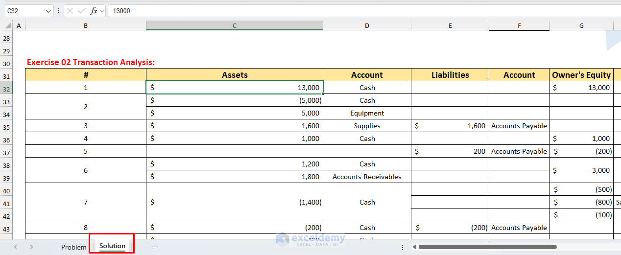
Your comment is not clear. Can you explain it in detail?
Regards
ExcelDemy
Hello Blemish Go,
To get the ISO week number and the correct year (so that 1-Jan-2027 is shown as 2026w53), you need to follow the ISO 8601 standard. Excel’s built-in WEEKNUM function alone won’t handle the year rollover correctly for ISO weeks, but you can use the ISOWEEKNUM function (available in Excel 2013 and later) plus an extra formula for the ISO year.
Steps:
Week Number:
Use =ISOWEEKNUM(A1) where your date is in cell A1.
ISO Year:
Use this formula for the ISO week year (paste in any cell):
=A1-WEEKDAY(A1,2)+4
Then extract the year from that result:
=YEAR(A1-WEEKDAY(A1,2)+4)
Combine both for the ISO format:
=YEAR(A1-WEEKDAY(A1,2)+4) & “w” & TEXT(ISOWEEKNUM(A1),”00″)
For 1-Jan-2027, this will correctly return 2026w53.
Regards
ExcelDemy
Hello Jenand,
You are most welcome. Glad to hear that your issue is solved now. Thanks for your feedback and appreciation.
Regards
ExcelDemy
Hello Vanessa,
You can achieve this by using the VLOOKUP function with a helper column to combine the first and last names for an exact match. Here’s how you can do it:
Step 1: In both worksheets, create a new column (for example, Column D) that combines Last Name and First Name. Use this formula in cell D2 of both sheets:
=A2 & ” ” & B2
Step 2: Now, in Worksheet 1 (let’s say in cell C2), use the following formula to bring the location from Worksheet 2:
=VLOOKUP(D2, ‘Worksheet2’!D:C, 3, FALSE)
‘Worksheet2’!D:C assumes you have the combined names in Column D and location in Column C in Worksheet 2.
Adjust the column references as needed. It checks for an exact match of combined first and last names in both sheets and returns the location from Worksheet 2.
Regards
ExcelDemy
Hello Ryan,
Thank you for your feedback! If the macro isn’t running automatically, you’ll want to use a worksheet or workbook event to trigger it. For example, you can place the macro call inside the Worksheet_Change event (for changes in a specific sheet) or in the Workbook_Open event (to run when the file opens).
Example (run automatically when data changes in Sheet1):
1. Right-click the Sheet1 tab and choose View Code.
2. Paste this code in the code window:
Private Sub Worksheet_Change(ByVal Target As Range)
Call SyncRowsBasedOnMultipleDates
End Sub
Now, whenever you change any data in Sheet1, the macro will run automatically.
Regards
ExcelDemy
Hello Mebratu Merdekios,
If you have any query or issue let us know. We try our level best to solve your issue.
Regards
ExcelDemy
Hello Rob,
You’re welcome! Glad Method 1 worked for you. Excel can indeed be tricky sometimes.
Let me know if you run into any other issues!
Regards
ExcelDemy
Hello Rohit,
Sorry to hear that. Please ensure you have used valid email address. Also check the spam folder.
If everything is okay, after subscribing the Excel file automatically sent to your inbox.
You can try again,
“Download the Practice Files”
Then check your email immediately after to get the download links.
Best Regards
ExcelDemy
Hello A.King,
Thank you for your comment! The confirmation dialog that appears when merging cells in Excel is actually a built-in feature of Excel, not something new.
It usually pops up to warn users that merging cells will keep only the upper-left value and discard other data in the selected range.
If you want to avoid this dialog when using VBA, you can add a line like Application.DisplayAlerts = False before merging, and set it back to True afterward.
Regards
ExcelDemy
Hello Jennifer Enriquez,
Share your problem in ExcelDemy Forum. There you can upload images, Excel and etc.
Also brief your problem in detail.
Regards
ExcelDemy
Hello Jennifer Enriquez,
Share your problem in ExcelDemy Forum. There you can upload images, Excel and etc.
Also brief your problem in detail.
Regards
ExcelDemy
Hello Mohammed Nadim,
Thank you so much, for your kind and thoughtful feedback!
We’re truly grateful that you found the article clear, well-structured, and easy to follow. It’s always our goal to make complex Excel tasks more approachable, and it’s encouraging to know the step-by-step explanation helped simplify things for you.
Your appreciation means a lot to me and the entire ExcelDemy team. We’re committed to continuing to provide practical, valuable content to support learners like you.
Best wishes,
Shamima
Hello Misiko Purity,
You are most welcome. Thanks for your feedback and appreciation, It means a lot to us.
Keep exploring Excel with ExcelDemy.
Regards
ExcelDemy
Hello Paul,
You are most welcome. Thanks for your feedback and appreciation, It means a lot to us.
Keep exploring Excel with ExcelDemy.
Regards
ExcelDemy
Hello Jennifer Enriquez,
Thanks for reaching out. The discount formula you’re using =F5*IF(D5<1,0.03,0.05) looks correct and should calculate a 3% discount if the price is less than 1, and a 5% discount otherwise.
If it’s not working as expected, please double-check that the cells you’re referencing contain numbers (not text or empty values).
Also, make sure there are no extra spaces in the price or amount cells.
If you’re still having trouble, could you share more details or a screenshot of the issue? I’d be happy to help further!
Regards
ExcelDemy
Hello Matt Senko,
Thank you for your update. If you’re still getting the same syntax error, please check these points:
1. Correct Quotes: Make sure you are using straight single ‘ or double ” quotes (not curly quotes or backticks) in your expression.
2. OData Query Format: If you are using OData filter queries (common in Power Automate when filtering SharePoint or similar), the syntax should look like this:
Deadline eq ‘2024-10-03T00:00:00Z’
Or, if your column is of type Date and you’re only comparing the date (not time), try:
Deadline eq 2024-10-03
But most APIs expect the value in single quotes and sometimes require the full date-time with “T” and “Z” for UTC.
3. Field Name: Double-check that the column name Deadline is spelled exactly as it appears in your source (case-sensitive and no extra spaces).
4. Connector-specific Format: If you’re using SharePoint, the correct OData query is:
Deadline eq ‘2024-10-03T00:00:00Z’
If you are querying a table with just a date (not datetime), use:
Deadline eq ‘2024-10-03’
5. Spaces: Make sure there are no extra spaces in the query string.
If you’re still having issues, could you please share a screenshot of your filter query or let us know which connector/service you’re using in Power Automate? This will help to give you a more targeted solution.
Let me know how it goes!
Regards
ExcelDemy
Hello Courtney Hoffman,
How to update it to 800 months:
1. Search for “804” in the worksheet—press Ctrl + F, type 804, and go through each result.
2. Replace each instance of 804 with 800 (your FRA of 66 years 8 months, i.e. 66×12 + 8).
3. This ensures all formulas that calculate based on FRA will now use 800 months.
The main places you’ll find it:
1. The “Total Months” calculation row (Method 2).
2. Any formulas referencing months-based FRA, particularly in cumulative benefit comparisons (Methods 4–6).
Just swapping 804 → 800 in those formulas will adjust the break‑even analysis to reflect your actual FRA.
Let me know if you’d like me to walk through one specific example or cell!
Regards
ExcelDemy
Hello Ryan,
Thank you so much for your feedback! If you have multiple columns that could contain dates (for example, 6 different columns), you just need to adjust the VBA code so that it checks all those columns in each row. If any of those columns has a date, the row will go to Sheet2; if none have dates, the row will go to Sheet3.
Here’s how you can update the macro:
Just update the dateCols array to match the columns you’re using for dates.
Let me know if you need help customizing this further!
Regards
ExcelDemy
Hello Neil Homes,
In Excel, you can place data labels above the bars by setting their position to “Outside End.” Here’s how:
1. Click on your chart to select it.
2. Click the plus (+) icon next to the chart or go to Chart Elements >> select Data Labelswww.
3. Choose Outside End from the options.
This will automatically place the data labels just above the bars, near the edge, without needing to move each label manually.
If you still want the labels closer or need finer adjustment, unfortunately, Excel does not offer a setting for custom spacing, you would have to adjust them individually. But for most cases, “Outside End” works well!
Regards
ExcelDemy
Hello Ryan,
Great question! What you’re describing is possible in Excel, but it usually requires a combination of formulas or VBA (macros), since you want the data on Sheet 2 and Sheet 3 to automatically update based on whether there is a date in the row on your master sheet (Sheet 1).
Use Formulas (For Viewing Only, Not for Actual Row Copy)
If you just want to display rows from the master sheet on Sheet 2 and Sheet 3 (without actually copying and removing rows), you can use formulas like FILTER (in Excel 365/2021), or helper columns with IF and INDEX/MATCH in older versions.
For Sheet 2 (rows with dates):
=FILTER(‘Sheet1’!A2:D100, ISNUMBER(‘Sheet1’!B2:B100))
(Assuming the date is in column B. Adjust range as needed.)
For Sheet 3 (rows without dates):
=FILTER(‘Sheet1’!A2:D100, NOT(ISNUMBER(‘Sheet1’!B2:B100)))
VBA Approach
This VBA solution will copy (not move) the relevant rows to Sheet2 and Sheet3 each time you make a change in the Master sheet. Sheet2 and Sheet3 are refreshed every time, so they always show the correct filtered rows.
1. Press ALT + F11 to open the VBA editor.
2. Insert a new module (Right-click on any object in the Project Explorer > Insert > Module).
3. Copy and paste the following code into the module.
Auto-Run Macro When Master Sheet Changes
To make the macro run automatically when you change anything in the master sheet:
1. In the VBA editor, double-click on Sheet1 (or your master sheet).
2. Paste this code:
Regards
ExcelDemy
Hello Syed,
Thank you so much for your kind words! I’m glad you found the explanation helpful. Yes, you can use the XLOOKUP formula together with the FILTER function to skip multiple empty cells in a row and extract only the values.
For example, if your data is in the range A2:F2, you can use the following formula to return only the non-empty values:
=FILTER(A2:F2, A2:F2<>“”)
This formula will give you a list of all non-blank values from the row. If you need to use XLOOKUP to match and retrieve specific non-blank values from another list, you can combine these functions based on your exact scenario.
Regards
ExcelDemy
Hello Steve,
Thank you for your comment and for pointing this out!
Actually, the section to download the Excel Formulas Cheat Sheet PDF & Excel Files is located right on the first page of the article. You’ll find it under the heading:
“Download the Excel Formulas Cheat Sheet PDF and Excel Files”
There, you’ll see a form asking for your First Name and Email Address—just above the blue “Download” button. Once submitted, you’ll receive access to the files.
If that section isn’t visible to you, it might be due to:
1. An ad blocker or privacy extension
2. Browser caching issues
3. Disabled JavaScript
We recommend refreshing the page or trying in incognito/private mode. If it still doesn’t work, feel free to contact us.
Best regards,
ExcelDemy
Hello Shell,
Thanks for your comment! If you’re seeing blank cells getting highlighted along with overdue dates, you can adjust the formula to ignore blanks. Try this version in Conditional Formatting:“”)
=AND(A1
This formula checks if the date is before today and not blank, so it will skip empty cells. Let me know if it works or if you’d like a specific example based on your data layout!
Regards
ExcelDemy
Hello Ava,
You’re welcome! To enter the selected date from the CalendarForm into the active cell, you need to add some code to your CalendarForm. Here’s how you can do it:
In your CalendarForm code, after the user selects a date (for example, when they click on a date or an OK button), add this line:
Make sure that “Calendar1” matches the name of your calendar control on the form.
So, your event (for example, a button click) in the form might look like this:
This will insert the selected date into the active cell when you select a date from the CalendarForm.
Regards
ExcelDemy
Hello Irina,
Please check your email inbox or spam folder. After subscribing the cheat list is automatically sent to your email address.
Or you can follow the steps again,
go to the “Download Excel Formulas Cheat Sheet PDF & Excel Files” section of this post and enter your email address.
Then check your inbox/spam folder to get the Excel file.
Regards
ExcelDemy
Hello PF,
Thank you for your valuable input! Adding 365 days isn’t the best way to add full years to a date, especially around leap years. However, there are some specific scenarios where Method #1 can be useful.
For example, if you need to calculate a fixed interval of exactly 365 days—such as certain types of reminders, subscriptions, or analytical periods—then this approach works well.
In these cases, you’re looking for a span of “365 days” rather than the same date in a future year.
For most situations where the goal is to land on the same calendar date in the future, using EDATE or DATE is definitely the better and more accurate choice. Thank you again for your feedback. Discussions like these help to improve the quality and usefulness of our content!
Regards
ExcelDemy
Hello Annie Hall,
You can add another conditional formatting rule with a formula to highlight dates that are within 6 months of turning 3 years old.
Try this formula:
=AND(TODAY()>=EDATE(A1,30), TODAY()
This assumes your date is in cell A1.
Explanation:
EDATE(A1,30) gives the date that’s 2.5 years (30 months) after the original date.
EDATE(A1,36) is exactly 3 years later.
The formula checks if today is between 2.5 and 3 years after the date, which means within 6 months of being 3 years old. Just adjust the cell reference as needed for your range. Let me know if you need step-by-step instructions!
Regards
ExcelDemy
Hello Alireza Bagheri,
You are most welcome. Thanks for your feedback and appreciation. Keep exploring Excel with ExcelDemy!
Regards
ExcelDemy
Hello Manohar,
Hope you are doing well.
You are most welcome. Keep exploring Excel with ExcelDemy!
Regards
ExcelDemy
Hello Kal,
Absolutely! Here’s a simple step-by-step guide you can follow to attach your Excel worksheet to an email:
1. Open your email program (like Gmail, Outlook, Yahoo, etc.).
2. Start a new email (look for a button that says “Compose” or “New Message”).
3. Click on the paperclip icon (this is the “Attach” button).
4. A window will open showing your computer files. On the left side, click “Desktop” (since you saved your Excel file there).
5. Find and click your Excel file (it should end with .xlsx or .xls).
6. Click the “Open” or “Attach” button (usually in the bottom right of the window).
7. You’ll see your file attached to your email.
8. Now you can type your message and click Send.
If you get stuck, just let me know exactly where and I’ll walk you through it!
Regards
ExcelDemy
Hello Johan Stroman,
You’re very welcome, Johan! We’re glad you found the summary helpful and easy to use. If you have any questions or need more tips on using Excel for financial statements, feel free to ask. Thanks for your kind words!
Keep exploring Excel with ExcelDemy!
Regards
ExcelDemy
Hello Manohar,
Thank you so much for your kind words! I’m glad you found the tutorial helpful. To become a better data visual designer, I recommend practicing regularly with different types of datasets and exploring various chart types in Excel, such as maps, scatter plots, and pivot charts.
Try to tell a clear story with your visuals and always keep your audience in mind. Reviewing examples of effective dashboards and visualizations online can also be very inspiring. Lastly, don’t hesitate to experiment with colors, layouts, and design elements to find your own style.
Explore our Excel Charts category to learn more about visualizations.
Best wishes on your learning journey!
Regards
ExcelDemy
Hello Eric Smith,
Thank you for sharing your method. Saving the file as a CSV and then reopening it in Excel is indeed a quick way to convert text-formatted numbers back to numeric values, especially when dealing with large datasets.
As you mentioned, some formatting may be lost, but it’s a useful workaround when standard Excel methods aren’t practical. Cheers!
Regards
ExcelDemy
Hello,
Thank you for pointing that out! Yes, the method shown in the article uses the ΔE from the 1976 (CIE76) formulation.
You are correct that the current industry standard is ΔE 2000 (CIEDE2000), which provides a more accurate measure of color difference.
For advanced applications, it’s better to use the DE 2000 calculation.
Regards
ExcelDemy
Hello Sunit,
To set a fixed email subject line in your VBA code, you just need to assign your desired subject text to the .Subject property. For example:
.Subject = “Your Fixed Email Subject Here”
Place this line in the section of your VBA code where you create the email, and every email sent will have the same subject line.
Regards
ExcelDemy
Hello Michael Seleanu,
You can achieve this by adding columns for the 50-day and 200-day moving averages using Excel’s AVERAGE formula, then use logical formulas to set cross-over flags. For example, to flag when the current price crosses above the 50-day moving average, you could use a formula like:
=IF([@[Current Price]] > [@[50-day MA]], “Crossed Above”, “”)
Similarly, compare against the 200-day MA for another flag. You can also use conditional formatting to highlight cross-overs visually in your table.
Regards
ExcelDemy
Hello Paul,
It sounds like your spreadsheet still has an Excel Table or some filter settings left over from when you used Queries & Connections. The “Column 1, Column 2…” labels usually appear when Excel creates a new table from an imported source.
A few things you can try:
Convert the Table Back to a Range:
1. Select any cell in the table (Row 1360, Columns A to AA).
2. Go to the Table Design tab >> click Convert to Range.
3. Confirm if prompted.
This should turn your table back to a normal range and remove the special “Column 1, Column 2…” headers.
Remove Filters:
1. Go to the Data tab.
2. Click Clear (next to the Filter button) to remove all filters.
3. Check if the headers disappear.
Delete Unwanted Rows: If you still have the “Column 1, Column 2…” row, you can simply select Row 1360 and delete it (right-click the row number > Delete).
About the Delete being greyed out: This usually means the connection is still in use, or the worksheet is protected.
Make sure: The table/range linked to the query is removed.
The sheet is not protected (Review tab > Unprotect Sheet).
Regards
ExcelDemy
Hello Savannah,
You are most welcome. Yes, you can achieve this easily by using an IF formula. For example:
=IF(A1=”YourValue”, “AutofillText”, “”)
This formula will autofill the cell only when cell A1 contains “YourValue”; otherwise, it’ll remain blank. Let me know if you need further clarification!
Regards
ExcelDemy
Hello Ronald Pagaduan,
You can use the SUMIF function with 3D referencing if your description and values are in the same cells across multiple sheets.
For example, if your sheets are named Sheet1, Sheet2, and Sheet3, and you want to add all amounts for a description in column A with values in column B, you can use:
=SUM(SUMIF(INDIRECT(“‘”&{“Sheet1″,”Sheet2″,”Sheet3″}&”‘!A:A”), “Your Description”, INDIRECT(“‘”&{“Sheet1″,”Sheet2″,”Sheet3″}&”‘!B:B”)))
Or, for many sheets, you might need a helper column or use Power Query to combine data first, then sum.
Regards
ExcelDemy
Hello Manohar,
Greetings! Thank you for your kind words. I’m glad the explanation was helpful for you. If you have any more questions about Excel or need further clarification, feel free to ask.
Best regards,
ExcelDemy
Hello Manohar,
Thank you for your kind words! I’m glad you found the tutorial helpful. Regarding your question about “Pre,” “Post,” and data labels in a waterfall chart:
Pre and Post are used to clearly show the starting and ending values in the waterfall chart. They help you see the initial amount before any changes and the final amount after all changes.
Data labels are used to display the exact values on each bar of the chart. This makes it easier to understand the amount for each step, whether it’s an increase or a decrease.
Using these elements together makes the waterfall chart more readable and helps users quickly see how each step contributes to the total change.
Regards
ExcelDemy
Hello Manohar,
Thank you for your question! The “Start Line” in column B is used as the base value for each bar in the stacked waterfall chart. It helps to position the rise (increase) and fall (decrease) segments correctly along the Y-axis, so the chart visually represents the cumulative effect.
If you use column B as the base and columns C and D as rise and fall, you’d need to make sure your chart is set up to stack these values in the correct order. The “Start Line” column specifically helps in showing the starting point for each change, making the chart easier to read.
Hope this helps! Let me know if you need more details.
Regards
ExcelDemy
Hello Brian Laursen,
The code provided in the article is still working as of now. If you’re experiencing any issues or need an updated version, please share more details, we will be happy to help!
Regards
ExcelDemy
Hello Brian,
If the formula only works in C7 but not in the other cells (C8:C16), please make sure you are using absolute references correctly in your formula, and that the ranges are set properly when you copy down. Sometimes, copying a formula down can change relative references, which may cause the formula not to work as expected.
Also, double-check that your list/range names are consistent and that there are no hidden spaces or formatting issues in your data.
If you still face issues, please share the exact formula you are using, so the community can help you debug it step by step!
Regards
ExcelDemy
Hello Jana,
Thanks for sharing your workaround! Since the standard methods didn’t resolve your issue, it might be related to specific workbook settings or perhaps a glitch within Excel itself.
Could you check if any macros or conditional formatting rules might be affecting row numbering when you add or switch tabs? Alternatively, testing this in a fresh workbook could help identify if the issue is file-specific.
Regards
ExcelDemy
Hello Ric Esh,
Thank you for sharing your perspective. In the context of comparing strings in Excel, the term “similar” is often used to describe how much two text values resemble each other, even if they are not exactly the same.
While “similar” can imply some differences, in Excel functions it refers to the degree of likeness between two strings, which might include both small and significant differences depending on the method used.
Regards
ExcelDemy
Hello Allison,
You are most welcome. Thanks for your feedback and appreciation. Glad to hear our examples is helpful and you liked it.
Keep exploring Excel with ExcelDemy!
Regards
ExcelDemy
Hello Mohammad Afzal,
Thank you for your feedback and appreciation. Glad you found the article helpful. If you have any questions about Power Query, Power Pivot, or Power BI, feel free to ask. Happy learning!
Regards
ExcelDemy
Hello Cire,
Thank you for your feedback! You’re correct—simply adding years by multiplying 365 days doesn’t account for leap years, which can make the result inaccurate over longer periods.
To accurately add years to a date (including leap years), you should use the EDATE or DATE function in Excel:
Use EDATE:
If your date is in cell A2 and you want to add 4 years:
=EDATE(A2, 12*4)
This will add exactly 4 years, taking leap years into account.
Use DATE:
If your date is in cell A2 and you want to add 4 years:
=DATE(YEAR(A2)+4, MONTH(A2), DAY(A2))
This also accurately adds years, even if there are leap years.
These methods are more reliable for date calculations over several years.
Regards
ExcelDemy
Hello Wendy,
Great question! To make the code dynamic so you don’t have to update the array size manually when your data changes, you can modify the code to automatically find the last row and last column of each sheet. This way, your search will always cover the entire data range, no matter how much you add or delete.
For example, you can replace any fixed range like A2:D20 with code that uses UsedRange or calculates the last row/column like this:
Now, searchRange will always include all your data, even if rows or columns are added or removed. So, you don’t need to edit the array size in your code every time your data changes, just use this dynamic approach!
Regards
ExcelDemy
Hello Gordon Meredith,
Absolutely, Gordon! Yes, Excel can do exactly what you described. You can apply a “rolling” or compounded inflation rate each year so that each year’s amount includes the inflation added to the previous year’s total.
Here’s how you can set it up:
1. Enter your current monthly budget in a cell, say B2.
2. In column A, list the years (Year 0 to Year 18).
3. In column B, calculate the new budget for each year using the formula:
3.1. For Year 0 (the starting year), just use your current budget.
3.2. For Year 1 and onward, use this formula (assuming 3.55% inflation):
=B2*(1+3.55%) for the first year, and then drag the formula down so each year multiplies the previous year’s value by 1.0355.
Example (assuming your budget is in B2):
Year 0: =B2
Year 1: =B3*1.0355
Year 2: =B4*1.0355
…and so on.
You can drag the formula down for 18 years, and Excel will show you how your budget grows each year with compounded inflation.
Regards
ExcelDemy
Hello Jana,
Yes, it is definitely possible to have a worksheet where each student’s report card appears one after the other, instead of showing only one student (like Henry) with multiple terms.
To do this, you can create a template for a single report card, then copy and paste it below for each student, updating the student’s details and marks accordingly. This way, you’ll have a continuous list of individual report cards—one after another—in the same worksheet.
If you are using formulas or references, make sure to adjust them for each section so they refer to the correct student data. You can also use Excel features like Page Breaks to make each student’s report card print on a separate page if needed.
Regards
ExcelDemy
Hello Nuva,
The “ByRef argument type mismatch” error usually means that the variable type you’re passing to a procedure (like a Sub or Function) doesn’t match the expected type in its definition. Even if the code looks correct, double-check these common causes:
Make sure the argument types match exactly between where you call the procedure and where it’s defined (e.g., String vs. Variant, or Range vs. String).
If you’re passing a cell reference, use Range as the argument type, not String.
For example, if your Sub is defined as Sub SaveData(ByRef cell As Range), but you call it with a string like SaveData(“A1”), that will cause this error. Instead, use SaveData(Range(“A1”)).
Regards
ExcelDemy
Hello Diva,
Thank you for your thoughtful comment and your interest in the advanced Excel dashboard tutorial. I’m glad you found it insightful!
To make your learning experience easier, I’ve attached a downloadable file with the sample dataset (Sales, Products, Customers, and Regions) as well as the complete dashboard solution. You can use this file to follow along step by step and practice building your own dashboard.
If you have any questions or need further assistance, please feel free to reach out. Happy learning!
Regards
ExcelDemy
Hello Flavio,
Good morning! Thank you so much for your kind words and for sharing your feedback!
I understand how useful it is to have a practice file to follow along. I’m happy to let you know that I’ve now attached a downloadable file containing both the sample dataset and the dashboard solution. You can use this file to practice and explore all the features demonstrated in the tutorial.
Thank you again for your support and encouragement. If you have any further questions or need more resources, feel free to let me know!
Regards
ExcelDemy
Hello Hannes,
Good morning! Yes, I can definitely assist you with that.
Step-by-Step Guide to Build the 24×7 Shift Roster in Excel:
Step 1: Set Up the Date Headers
1. In Row 1 (starting from B1), enter all the dates for the month horizontally (e.g., B1:AF1 for a 31-day month).
2. Format them as dd-mmm.
Step 2: List Employees Vertically
In Column A (starting from A2), list all 35 employee names (e.g., A2:A36).
Step 3: Define Shift Codes
Use the following codes:
D = Day shift
N = Night shift
O = Off
Step 4: Create Rotating Pattern
In another sheet or helper table, define a base pattern (e.g., 5D, 3O, 5N, 3O = 16-day cycle). Repeat this pattern across the month for each employee, staggered so shifts rotate evenly.
Example for Employee 1:
D, D, D, D, D, O, O, O, N, N, N, N, N, O, O, O …
Shift each subsequent employee’s pattern by a few days to ensure:
No overcrowding on the same shift
Balanced 15 Day / 9 Night coverage
Step 5: Use Formulas to Apply Patterns
Use Excel formulas like =INDEX() or =OFFSET() to fill in shifts for each day, repeating the 16-day cycle across the month.
Example formula for B2:
=INDEX($Z$2:$AO$2,MOD(COLUMN(B2)-2,16)+1)
Where Z2:AO2 contains the 16-day pattern for that employee.
Step 6: Count Shifts Per Day
Below the roster table (e.g., row 38+), insert formulas to count:
How many “D” per day:
=COUNTIF(B2:B36, “D”)
How many “N” per day:
=COUNTIF(B2:B36, “N”)
Use conditional formatting to highlight if the count isn’t 15 (for day) or 9 (for night).
Step 7: Optional – Add Conditional Formatting
Use color coding:
Green for “D”
Blue for “N”
Gray for “O”
This improves readability.
Regards
ExcelDemy
Hello Phelim Murnion
Thanks for your feedback! Method 3 should work if the steps are followed correctly, but it may depend on your Excel version or settings. Could you please share more details about the issue you’re facing? I’d be happy to help troubleshoot it.
Regards
ExcelDemy
Hello Sara,
Yes, you can achieve this with a bit of VBA. Excel doesn’t support adding form controls like checkboxes conditionally through formulas, but you can use a simple macro to loop through a range and add checkboxes next to cells that contain text.
Here’s a sample VBA code that adds checkboxes conditionally next to cells only if the adjacent cell contains text:
1. Press Alt + F11 to open the VBA Editor.
2. Insert a new module (Insert > Module).
3. Paste the code and run it (F5) while your desired worksheet is active.
Regards
ExcelDemy
Hello Daryl Fagala,
Thank you for the feedback! A practice workbook with sample data would make it easier to follow along. Attached the downloadable file to enhance the learning experience. Appreciate your suggestion!
Regards
ExcelDemy
Hello Ryan,
Thank you for the follow-up! Based on your needs—multiple sites with varying numbers of day and night shift employees (from 1 to 4) you can prepare a scalable Excel roster template where:
Roster Dates Setup:
1. In Row 1 (starting from Column B), enter the dates from the 26th of the previous month to the 25th of the current month.
2. Use a formula like this in cell B1:
=DATE(2025,6,26)
3. Then drag across 30 cells to reach the 25th of the next month.
Master Shift Pattern:
1. In a row (e.g., Row 3), input the repeating 7-day pattern: D, D, D, N, N, X, X
2. Use this formula in Row 4 for each date column (starting from B4):
=INDEX($B$3:$H$3,MOD(COLUMN()-COLUMN($B$3),7)+1)
3. This will repeat the pattern every 7 days.
Apply to Employees:
1. Copy Row 4 for each employee’s row to apply the same pattern.
2. If you want each employee to start on a different day in the cycle, adjust the MOD(…)+1 portion accordingly.
Scalability for Multiple Sites:
1. You can group employees by site using separate blocks or color codes.
2. Just replicate the employee section and change headers for each site.
3. To scale up or down, simply copy or delete rows as needed.
You’ll be able to adjust the number of employees per site easily, thanks to dynamic formulas.
Regards
ExcelDemy
Hello Danley,
That’s a great tip! Pressing F9 is definitely quicker for recalculating the whole sheet. The calculate button is handy when you want more control or need to limit recalculation to specific areas.
Regards
ExcelDemy
Hello Jon,
You’re very welcome! Glad to hear it saved your time. Excel wins again!
Let us know if you want more tips like this. Keep exploring Excel with ExcelDemy!
Regards
ExcelDemy
Hello Avinash,
Excel skills are definitely essential for most accounting jobs! From financial analysis to budgeting and reporting, Excel is a key tool in the accountant’s toolkit. Let me know if you’d like tips or resources to get started!
Regards
ExcelDemy
Hello Vishal Kapadiya,
You are most welcome. Thanks for your feedback and appreciation. Glad to hear that our article is helpful to you.
Keep exploring Excel with ExcelDemy!
Regards
ExcelDemy
Hello Ryan,
For your setup, where the roster runs from the 26th of the previous month to the 25th of the current month, you’ll need to adjust the date formulas in the template so the start date is always the 26th, and the end date is the 25th of the next month.
For the repeating pattern (like D, D, D, N, N, X, X), you can set up a “pattern” input cell or row for each employee (or as a master pattern), and then use formulas to repeat that pattern across the days.
If you want to change the pattern and have it auto-update for all employees, you can use a single reference pattern row and have each employee’s shift row pull from that, repeating every 7 days.
If you’d like, I can walk you through the formulas or even share a sample file. Let me know your preferred shift patterns and how many employees you have, and I can help you build a customized template!
Regards
ExcelDemy
Hello Rahul,
Thank you so much for your valuable feedback! You’re absolutely right, knowing how to make predictions after performing regression is essential for applying it effectively.
Once you’ve used Excel’s Data Analysis Toolpak to perform linear regression, you’ll receive an output with coefficients like this:
Intercept (α)
X Variable 1 Coefficient (β)
Let’s say the regression equation from your output is:
Y = α + βX
Step-by-Step to Make Predictions:
1. Identify Coefficients: From the regression output table:
Intercept = 2.5
X Coefficient = 1.8
So, the regression equation is:
Predicted Y = 2.5 + 1.8 * X
Create a Column for New X Values:
1. Suppose in column F (F2:F6), you input new X values (e.g., sales, height, etc.)
2. Use a Formula to Calculate Predicted Y:
3. In column G, enter the prediction formula:
=2.5 + 1.8 * F2
Drag this formula down to apply it for all new X values.
Regards
ExcelDemy
Hello Andrew,
You are most welcome. Glad to hear that Text to Column method worked for you. Keep exploring Excel with ExcelDemy!
Regards
ExcelDemy
Hello Sharon Polman,
Thank you for your feedback! You’re absolutely right, hiding columns can get messy, especially when the selected columns aren’t adjacent. A better alternative for printing non-contiguous columns (like Name, Credit Card, January, and December) is to copy those specific columns into a new sheet just for printing purposes.
That way, you can arrange them exactly how you want, avoid the clutter of hidden columns, and keep your original worksheet intact. If you’re frequently printing custom views, using the Camera Tool or setting up a custom print area in a helper sheet can also streamline your workflow. Appreciate your input!
Regards
ExcelDemy
Hello Ines ,
If you’re getting errors while pulling specific project titles into a summary table, it could be due to the formula setup or data range selection. For this task, the FILTER function (available in Excel 365 and Excel Online) is very effective. You can use a formula like:
=FILTER(A2:B41, ISNUMBER(MATCH(A2:A41, {“Project1″,”Project2″,”Project3″,”Project4”}, 0)))
1. Replace A2:B41 with your actual data range.
2. Update {“Project1″,”Project2″,”Project3″,”Project4”} with your specific project titles.
If you’re not using Excel 365, you may need to use a combination of INDEX and MATCH with helper columns. Double-check your ranges and project names for typos. If you share the exact error message or formula, I can help further!
Regards
ExcelDemy
Hello Irfan Zuberi,
hank you so much, Irfan! Your kind words truly mean a lot. I’m glad you found the article helpful. If you have any more questions or need further tips, feel free to ask.
Regards
ExcelDemy
Hello Arun Kumar,
Thank you for reaching out! It’s great that you’re working on a Power BI project to showcase your skills.
For practice datasets, you can explore our Excel Sample Data (Free Download 13 Sample Datasets) article, which provides a variety of data you can use for your sales dashboard.
To help you get started with Power BI, check out these Exceldemy resources:
Getting Started with Power BI
Power Bi Article List
These guides will walk you through extracting data, importing it into Power BI, building interactive dashboards, and showcasing your work for your resume and LinkedIn.
If you need any specific help with Power BI features or your project workflow, feel free to ask! Best of luck with your project and your career!
Regards
ExcelDemy
Hello Syed Mustfa,
Wa alaikum assalam! Thank you for your message.
You can find more practice data with solution sheets in the articles listed above. All of the article includes solution sheet. You will need to download it from articles.
Regards
ExcelDemy
Hello Erin,
Yes, you can use a formula to count how many times “A” appears in a range of cells. If the values are stored in a range like A1:A20, and each cell may contain multiple letters (e.g., “AB”, “AAB”), you can use this array formula (press Ctrl+Shift+Enter if you’re using an older version of Excel):
=SUM(LEN(A1:A20)-LEN(SUBSTITUTE(A1:A20,”A”,””)))
This formula calculates how many times “A” appears across the range. It should return 11 if there are exactly 11 “A”s in total.
Regards
ExcelDemy
Hello Jack,
To display the calendar in all cells, you need to use VBA to trigger the calendar whenever any cell is selected. Here’s how you can do it:
1. Open the VBA editor (press Alt + F11) and insert the calendar UserForm if you haven’t already.
2. In the sheet module (for example, Sheet1), use the Worksheet_SelectionChange event. This code makes the calendar pop up every time you select a cell on the sheet.
Replace CalendarForm with the actual name of your UserForm.
If you want the calendar to appear only for specific cells (e.g., only in column A), you can adjust the code like this:
Make sure the calendar form is set up to enter the selected date into the active cell, so when a user picks a date, it’s inserted into the cell they clicked.
Note: Showing the calendar for every cell might be intrusive, so you may want to limit it to certain columns or a range.
Explore this article: How to Insert Calendar in Excel Cell
Regards
ExcelDemy
Hello Dear,
Sama-sama. Thanks for your appreciation and feedback. Keep exploring Excel with ExcelDemy!
Regards
ExcelDemy
Hello Shane V,
Thank you for sharing your thoughts! If you change the “Apply to” selection in the conditional formatting rules, you can target individual cells or columns, not just rows. This makes it possible to highlight multiple text values in any range, not only across entire rows. Hope this helps!
Regards
ExcelDemy
Hello Luisa ,
Great questions! Here’s how you can address each of your points:
Color the cells based on selected option:
You can use Conditional Formatting instead of VBA to color the cells dynamically based on selection. However, if you want to use VBA, you’ll need to handle the Worksheet_Change event. Here’s a simple example:
Apply dropdowns across multiple tables/sheets:
You’ll need to run the MultipleDropDownList sub for each sheet and range combination. You can loop through sheets or define specific ones like this:
Define multiple non-contiguous ranges:
You can call the function separately for each range:
Regards
ExcelDemy
Hello Ayub,
You are most welcome. Thanks for your feedback and appreciation. Glad to hear that our assistance helped you to learn Excel account.
Regards
ExcelDemy
Hello Darlene,
It sounds like you might be using the mobile or tablet version of Excel, which has a more limited set of features compared to the desktop version. The Data tab in Excel for Android or iOS often lacks advanced tools like Data Validation, What-If Analysis, or Get & Transform (Power Query).
To access the full range of Excel features, including the complete Data tab, you’ll need to use the desktop version of Excel (Windows or Mac) with a full Microsoft 365 subscription.
Regards
ExcelDemy
Hello Jonathan,
With Method 3 (using “Get Data from Folder”), Power Query will combine all your files into a single table by default, which puts everything into one sheet. If you want to keep each workbook’s data on a separate sheet, you’d need to load each file individually or modify the query to split them.
Unfortunately, there isn’t a built-in option to automatically load each file into its own separate sheet when importing from a folder.
You’d have to either repeat the process for each file or use VBA or a custom Power Query solution to separate them after loading.
Custom Power Query Solution:
1. Go to Data → Get Data → From File → From Folder.
2. Select the folder containing the files.
3. Click Transform Data.
4. Now in Power Query: You’ll see a table listing all files.
5. Do not click Combine.
6. Right-click the binary link under the Content column >> select Add New Query (click on each cell manually).
7. This opens that file as a new separate query. Rename the query as needed.
8. Repeat this for all files.
Regards
ExcelDemy
Hello Genive Fernhout,
To extract cell A6 and B15 from each sheet into columns A and B of your first sheet, you can use a simple VBA macro. Here’s how:
1. Press Alt + F11 to open the VBA Editor.
2. Insert a new module: Insert > Module.
3. Copy-paste the following code:
Run the macro: Click Run or press F5.
This script loops through each sheet (excluding the first one), collects the values from cells A6 and B15, and pastes them into columns A and B of the first sheet.
Regards
ExcelDemy
Hello Kevin,
You are most welcome. Thanks for your feedback and appreciation. Keep exploring Excel with ExcelDemy!
Regards
ExcelDemy
Hello Akash Mathur,
To create dependent drop-downs (also called cascading drop-down lists) in Excel—so that selecting “Tablet” in the Category drop-down shows only related items (Acer, Dell, HP) in the Item drop-down—you can use named ranges and Data Validation with the INDIRECT function.
Steps to do it:
1. Create a unique list for Categories (e.g., Tablet, Hardware).
2. Create separate lists for each category’s items (e.g., a list of Tablet items: Acer, Dell, HP).
3. Name each item list exactly as the Category (e.g., name the Tablet items range “Tablet”).
4. Add Data Validation to the Category cell with the category list as the source.
5. Add Data Validation to the Item cell with the formula =INDIRECT(CategoryCell) as the source (replace CategoryCell with the actual cell reference).
Now, when you pick “Tablet” in the Category drop-down, only Acer, Dell, and HP will be available in the Item drop-down.
We also have other articles regarding dependent dropdown, you can explore these articles:
How to Create a Dynamic Dependent Drop-Down List in Excel
Excel Dependent Drop Down List (Create with Easy Steps)
Regards
ExcelDemy
Hello Ira Wati,
Your comment is not clear. Could you please describe your issue, if you need more help or have any questions about recovering Excel file passwords.
Feel free to ask. Have a great day!
Regards
ExcelDemy
Hello Usman,
You can download it from here: How to Build a Power BI Dashboard from Excel PivotTables and Charts
Regards
ExcelDemy
Hello Tolani,
You are most welcome. Thanks for your feedback and appreciation, it means a lot to us. Keep exploring Excel with ExcelDemy!
Regards
ExcelDemy
Hello Muhammad Q Naeem,
You are most welcome. Solved your issue, hopefully it will work.
Regards
ExcelDemy
Hello Muhammad Q Naeem,
When using SUMIFS to sum values greater than 121 (e.g., for an aging bucket “>121”), make sure your formula uses the correct criteria syntax. For example, if your “Aging” column is Column A and your values are in Column B, your formula should look like:
=SUMIFS(B:B, A:A, “>121”)
Common issues: Check that the values in your “Aging” column are actual numbers, not text. If they are text (e.g., “>121” as a label), SUMIFS won’t match them as numbers.
For aging analysis, create a helper column that actually calculates the numeric age (e.g., days overdue). Then, use SUMIFS on that column.
Example: If you have a calculated column for “Days Overdue,” your formula for the “>121” bucket should be:
=SUMIFS(B:B, C:C, “>121”)
(where C:C is your numeric “Days Overdue” column.)
If your bucket is a text like “>121”, use SUMIF with the bucket label:
=SUMIF(A:A, “>121”, B:B)
But the best approach is to calculate days overdue as numbers, then use SUMIFS with numeric criteria.
Regards
ExcelDemy
Hello Kabeli,
If you want to count how many times products were delivered to each country using VBA (with your delivery country codes, e.g., Canada = 011A, Germany = 012B, etc.), you can use a VBA script with a Dictionary. Here’s how you can do it with the same dataset:
How it works:
1. This code loops through the column with country codes and counts how many times each country appears.
2. The result will be listed in columns C and D, showing each country code and its delivery count.
3. Just change the column references or sheet name as needed.
Regards
ExcelDemy
Hello Vince,
Thank you for your feedback! I’m glad the guide helped you extract and work with your phone call and SMS records.
Yes, enabling the Developer option is often essential for properly importing and parsing XML files otherwise, as you noticed, everything can end up on a single line.
Appreciate you sharing your experience, and if you have any other questions or run into more tricky files, feel free to ask!
Regards
ExcelDemy
Hello Kim Tran,
Thank you for your follow-up! Yes, you are correct—Excel’s Data Validation does not handle references to external workbooks, and this is a built-in limitation of Excel, not just a step missing from the tutorial. Even when using named ranges, Data Validation will show the error if the range is in a different (closed) workbook.
Yes, this solution was tested, and the drop-down will only work if both workbooks are open at the same time. However, as soon as you close the source workbook, the drop-down list will break and show the error you mentioned.
Remember:
Data Validation can’t reference external workbooks reliably.
Best practice: Move or link your source list into the same workbook, or use Power Query or VBA to automate updating the list as needed.
Regards
ExcelDemy
Hello Kim Tran,
Excel’s Data Validation does not support referencing ranges from another workbook unless both workbooks are open at the same time. If the source workbook is closed, you’ll get the error: You may not use references to other workbooks for Data Validation criteria.
Here are a few workarounds:
Keep Both Workbooks Open: The drop-down list will work if both the source and target workbooks are open. But this isn’t always practical.
Copy the List into Your Current Workbook: The most reliable way is to copy the list/range you want to use into a (possibly hidden) sheet in the same workbook where you want the drop-down.
Use Power Query or VBA: With Power Query, you can import data from the other workbook and keep it refreshed. With VBA, you can create a macro to update the list as needed.
Unfortunately, referencing another workbook directly in Data Validation only works when both files are open. For a permanent solution, it’s best to have your list inside the same workbook.
Regards
ExcelDemy
Dear Atikah,
To obtain your required format please follow the following simple steps:
From your Excel Workbook, press ALT + F11 to open Visual Basic Editor.
Insert a module.
Paste the following code:
Now, return to your worksheet. Type in the following formula in the cell where you require the output and press Enter key.
=NumberToWords(B5) & ” Taka Only”
Here, B5 indicates the reference of the cell where you have the input number.
I hope this solution will be sufficient for your requirements. Let us know your feedback.
Regards,
ExcelDemy
Hello Patrick Raimond,
Great observation! Yes, it can be a bit confusing, ISBLANK only returns TRUE if a cell is truly empty, not if it contains a formula like =””.
In those cases, checking = “” directly, as you did, is the best approach. Thanks for sharing your solution, this tip will definitely help others who run into the same issue!
Regards
ExcelDemy
Hello Vpergl,
Thank you for sharing this great tip! Yes, with Excel 365 and later, the new dynamic array functions like FILTER, MAP, and especially the REGEXTEST function make it much easier to filter data using regular expressions—no VBA required.
Your formula is a perfect example of how powerful these new functions can be for pattern-based filtering. For anyone using Excel 365, this is definitely the preferred, modern way to achieve RegEx filtering. Thanks again for adding this valuable information!
Regards
ExcelDemy
Hello Monday Kolawole,
You are most welcome. Thanks for your feedback. Keep exploring Excel with ExcelDemy!
Regards
ExcelDemy
Hello Muhammad Q Naeem,
By default, Pivot Tables sort column labels alphabetically, which places “>120” first. To fix this and show the aging buckets in logical order (e.g., “0-30”, “31-60”, …, “>120”), follow these steps:
1. Right-click any column label in the Pivot Table.
2. Click Sort > More Sort Options.
3. Choose Manual and then drag the “>120” column to the end.
Alternatively, create a custom list for aging categories (e.g., “0-30”, “31-60”, “61-90”, “91-120”, “>120”) and use it in your Pivot Table sort settings:
1. Go to File > Options > Advanced > General > Edit Custom Lists.
2. Add your desired order, then sort by that list.
This will ensure the aging columns appear in the proper sequence.
Regards
ExcelDemy
Hello Chan Mau Yin,
It seems like the VLOOKUP inside your ISNUMBER is returning an error or text, not a number that means ISNUMBER(…) is evaluating to FALSE, and that’s why your formula always returns TRIM(MID(…)).
To fix this, make sure the 3rd column of ‘Table 1’!$A$4:$P$46 actually contains numeric values (not text numbers). Also, instead of using ISNUMBER(VLOOKUP(…))=TRUE, simplify the logic using IFERROR like this:
=IFERROR(VALUE(VLOOKUP(A5,’Table 1′!$A$4:$P$46,3,FALSE)), TRIM(MID(A5,2,2)))
This formula tries to return the VLOOKUP result; if it fails (error or not numeric), it falls back to TRIM(MID(…)).
Regards
ExcelDemy
Hello Andy Yang,
Thanks for the appreciation and feedback. You are right, we appreciate your effort. We updated the image.
Regards
ExcelDemy
Hello Mahin,
Sorry to hear that. Kindly check your spam folder also. You can download the Excel file free of cost just by providing your valid email address. To get the files go to the Top 100 MCQ of Excel section of this post and enter your email address. Then check your email immediately after to get the download links.
Please insert your name and email address then click on Download button.
Best Regards
ExcelDemy
Hello MJM,
You are most welcome. Thanks for your feedback and appreciation. Glad to hear that our article is helpful t you. Keep exploring Excel with ExcelDemy!
Regards
ExcelDemy
Hello Arashdeep Singh,
You are most welcome. Thanks for your appreciation. Keep exploring Excel with ExcelDemy!
Regards
ExcelDemy
Hello Greg,
Thanks for your comment! If your cells contain currency values formatted as text (like ‘$100’), the COUNTIF with wildcard may not work as expected.
Try using =SUMPRODUCT(–ISTEXT(range)) to count cells with any text, including currency-formatted text.
Also, make sure the cells are actually stored as text, not numbers with currency formatting.
Regards
ExcelDemy
Hello Cathy,
Glad to hear that. Excel is such a powerful tool, and there’s always something new to learn. Wishing you all the best as you continue to grow your skills!
ExcelDemy will be hear to help you.
Regards
ExcelDemy
Hello Aous Ymani,
To assign 8 technicians across 3 shifts per day with one day off per technician, you can use a rotating pattern in Excel. Here’s a basic idea:
Define the shifts: Morning (M), Afternoon (A), Night (N), and Off (O).
Create a pattern like this over a few days:
Day 1: M, A, N, O, M, A, N, O
Day 2: A, N, O, M, A, N, O, M
Day 3: N, O, M, A, N, O, M, A
Use a formula like this to rotate shifts across days (assuming A2 has Day 1 pattern and downwards):
=INDEX({“M”,”A”,”N”,”O”}, MOD(ROW()+COLUMN()-2,4)+1)q
You can adapt this to a full weekly/monthly schedule.
Regards
ExcelDemy
Hello Deliah,
You are most welcome. It’s our pleasure to help you with data entry files. To practice data entry you can explore the following articles. Download the files from the articles to learn and practice the exercises.
Excel Sample Data for Practice
Excel Data for Practice Free Download
Excel Practice Exercises PDF with Answers
Explore these categories you will find out more data entry practice here: Data Entry Practice Test & Quiz
Interview Questions with Excel Topics
MCQ Questions on MS Excel
To develop your skill from beginner to advanced level you can explore our Learn Excel page.
Regards
ExcelDemy
Hello Jkeej,
If Method 1 results in a tab-delimited .txt file when opened in Notepad, it’s likely because Excel defaulted to saving in a tab-delimited format (like .txt or CSV (MS-DOS)). To ensure commas are used as delimiters, make sure to:
Save the file explicitly as CSV UTF-8 (Comma delimited) (*.csv).
Check your system’s list separator setting (Control Panel > Region > Formats > Additional settings > List separator). It should be set to a comma (,), not a tab.
Try updating the list separator and saving again, this should fix the delimiter issue. Let me know if it helps!
Regards
ExcelDemy
Hello Zohra,
For a detailed mobile sales dataset suitable for an investor-ready dashboard, consider including the following columns:
Customer ID
Customer Name
Transaction ID
Date of Sale
Mobile Brand
Model
IMEI Number (optional)
Quantity
Unit Price
Discount
Total Sale Amount
Payment Method (Cash, Card, EMI, etc.)
Store Location / Sales Channel
Transaction Flow for Dashboard Design:
Leads/Visitors
Quotation Issued
Order Placed (with Customer ID)
Payment Processed
Device Delivered
Post-Sale Support / Warranty
Download the sample dataset: Mobile Sales Dataset.xlsx
Regards
ExcelDemy
Hello Frederik,
You’re very welcome! In Excel for the web (Excel Online), you can use Sheet Views to create personalized views for different users. This allows each person to filter or sort data without affecting others.
Here’s how to set it up:
1. Open the workbook in Excel Online.
2. Select the range or sheet you want to filter.
3. Go to the View tab > click New Sheet View.
4. Apply your filters or sorting, this will be saved just for you.
5. When others open the file, they’ll see the default view unless they switch to a different sheet view or create their own.
Each user can create and save their own Sheet View without impacting the main data display. Note that this works well for filters and sorting, hiding columns isn’t supported per user in Excel Online.
Regards
ExcelDemy
Hello Adrian,
Thank you for your detailed and insightful feedback! You’re absolutely right, the examples shown in the article are indeed EAN-8 codes with existing check digits, not the 12-digit base used to calculate an EAN-13 check digit.
We appreciate you pointing that out. We’ll update the examples accordingly to reflect a correct 12-digit input format for EAN-13 and 7-digit for EAN-8.
Also, your correction regarding the weighting order {1;3} is spot-on. In the standard EAN-13 calculation, the sum of digits in even positions is multiplied by 3, and the sum of digits in odd positions is used directly. The corrected array multiplication you provided using:
=MOD(-SUM(MID(TEXT(A1,”000000000000″),{1,3,5,7,9,11;2,4,6,8,10,12},1)*{1;3}),10)
is more accurate for generating the 13th digit from a 12-digit EAN-13 base number.
We’re updating the article to reflect these clarifications, and we truly appreciate your contribution to improving its accuracy!
Regards
ExcelDemy
Hello Guest,
You are most welcome. To calculate the weighted Average Handling Time (AHT) for a group (like John, Alex, and Sam), you need to weight each individual’s AHT by the number of calls they handled.
Use this formula:
=SUMPRODUCT(Number_of_Calls_Range, AHT_Range) / SUM(Number_of_Calls_Range)
For example, if:
John’s data is in row 2, Alex in row 3, and Sam in row 4
Column C = Number of Calls
Column G = AHT
Then the formula would be:
=SUMPRODUCT(C2:C4, G2:G4) / SUM(C2:C4)
This gives you the correct team AHT by accounting for how many calls each person handled. Let me know if you need help adjusting it for your sheet!
Regards
ExcelDemy
Hello Uju Ozu,
You are most welcome. Glad to hear that our article helped you to understand Excel functions easily. Keep exploring Excel with ExcelDemy!
Regards
ExcelDemy
Hello Fong,
Yes, you can definitely achieve that using Excel functions like VLOOKUP, INDEX-MATCH, or XLOOKUP (if you’re using a newer version of Excel). Based on your example, it seems you’re trying to:
Assuming:
Column A: Item names from Set 1
Column B & C: Corresponding values from Set 1
Columns E, F, G: Set 2 data (same structure)
You can use the following formulas:
To find matched name:
=IFERROR(INDEX($E$2:$E$100, MATCH(A2, $E$2:$E$100, 0)), “”)
To find matched values from Set 2:
=IFERROR(INDEX($F$2:$F$100, MATCH(A2, $E$2:$E$100, 0)), “”)
and similarly for the next column (Column G values).
To indicate match status (1 for match, blank otherwise):
=IF(COUNTIF($E$2:$E$100, A2), 1, “”)
This will align matched entries and leave the unmatched ones blank as you described.
Regards
ExcelDemy
Hello Yawa,
Solutions are given in the Excel file, attached in the Download section at the top of the article. Please download the Excel file to get the solutions.
Regards
ExcelDemy
Hello Swagmaster,
You’re right to point that out! Technically, most of the methods shown are shortcut-based techniques rather than a single keypress shortcut. The article focuses on efficient ways (like using Ctrl + Alt + V then selecting “Transpose”) but doesn’t mention a one-click shortcut because Excel doesn’t currently offer a dedicated keyboard shortcut for transposing.
Regards
ExcelDemy
Hello Walter P Anderson Jr,
You’re absolutely right! Dividends are a key part of stock evaluation. It would be very helpful if the article included data like dividend yield, payout ratio, ex-dividend date, and dividend per share. Fortunately, Excel’s Stocks data type can provide this info—just click the small insert data icon after converting the symbol. For example, to get the dividend yield, you can use a formula like
=A2.DividendYield (assuming your stock data is in cell A2).
Regards
ExcelDemy
Hello LN,
You are most welcome. Thanks for your feedback and appreciation. Glad to heart that our article helped you.
Keep exploring Excel with ExcelDemy!
Regards
ExcelDemy
Hello Derrek Quentin Davis,
You don’t need a separate software program—just use Microsoft Excel to begin calculating. The article includes a downloadable Excel worksheet you can use right away.
If you don’t have Excel, you can also use Excel Online (free with a Microsoft account) or Google Sheets to perform similar calculations.
Let me know if you need help getting started!
Regards
ExcelDemy
Hello Singa Menggala,
Thank you for your question and for using the practice file! To calculate income, the solution uses both the Problem sheet and the Reference Data sheet. Here’s a breakdown to help clarify the steps:
1. Determine Shift Type:
First, check which shift the employee worked (e.g., Morning, Evening, or Night) — this info is usually in the “Shift” column.
2. Find Pay Rate from Reference Data:
Go to the Reference Data sheet and find the corresponding hourly rate for that shift type.
3. Use a LOOKUP Formula:
In the Solution sheet, a formula like VLOOKUP or XLOOKUP is used to fetch the rate from the Reference sheet.
For example:
=VLOOKUP([@Shift], ‘Reference Data’!$A$2:$B$4, 2, FALSE)
This returns the hourly rate based on the shift.
4. Multiply by Working Hours:
Then multiply that rate by the number of hours the employee worked to get their income:
=Working_Hours * Shift_Rate
Let me know if you’d like a formula tailored to your version of Excel or a screenshot walkthrough.
Regards
ExcelDemy
Hello Franjo Tudjman,
I’m sorry to hear that the solution didn’t work for you. I understand how frustrating that can be. If you could let us know exactly which method you tried and what kind of data you’re working with, we’d be happy to help troubleshoot it further. Our goal is to make Excel easier for everyone, and your feedback helps us improve.
Looking forward to hearing more details so we can assist you better.
Regards
ExcelDemy
Hello Tela khan,
Hello, good evening! Thank you for your message.
You can find a ledger format in Excel at the following link:
Ledger in Excel (Complete Guideline)
How to Make a Ledger in Excel (Step-by-Step Guide)
Ledger in Excel
Please check these articles to download a ready template or learn how to create one yourself. Thank you!
Regards
ExcelDemy
Hello Mizanur t,
It looks like your message got cut off. Could you please resend it?
Regards
ExcelDemy
Hello Paul Wild,
It sounds like the columns C, F, and G in your table may have lost their formula consistency. In Excel tables, autofill relies on having a consistent formula pattern across the entire column. If a column has even one cell that’s different (blank or manually edited), Excel may stop automatically filling it in new rows.
Here’s how you can fix it:
Check for inconsistencies: Scroll through columns C, F, and G and make sure every cell above the new row has the correct formula. Correct any that are blank or manually changed.
Reapply the formula: Enter the correct formula again in the first cell of those columns and press Enter. Excel should then automatically fill the formula down to the entire column.
Convert and reconvert: If it’s still not working, you can temporarily convert the table back to a normal range (right-click the table → Table > Convert to Range) and then format it as a table again. This can reset autofill behavior.
Table Settings: Make sure that “Fill formulas in tables to create calculated columns” is enabled:
1. Go to File > Options > Proofing > AutoCorrect Options > AutoFormat As You Type tab.
2. Make sure “Fill formulas in tables to create calculated columns” is checked.
Regards
ExcelDemy
Hello again!
Thanks for the clarification! Since in your Build Log sheet the Date is in column A and the ID is in column B, you’ll need to slightly adjust the VLOOKUP.
In your Date Repair Built sheet (where you have the ID and want to bring the Date Built next to it), use this formula:
=VLOOKUP(A2, ‘Build Log’!B:A, 2, FALSE)
Important:
Notice that I reversed the range to B:A because VLOOKUP always searches in the first column of the range you specify. So here:
B:B is where it looks for the ID,
and A:A is where it pulls the matching Date Built.
Also, if you want to avoid errors for missing IDs, you can use:
=IFERROR(VLOOKUP(A2, ‘Build Log’!B:A, 2, FALSE), “Not Found”)
This will show “Not Found” instead of an error if the ID doesn’t exist in the Build Log.
Let me know if you want me to walk you through a full working example too! You’re doing great!
Regards
ExcelDemy
Hello Anne,
You’re right, Method 1 is not truly dynamic in real-time because it uses a named range based on the old GET.WORKBOOK function, which only updates when you force a full recalculation of the workbook. Simply refreshing or closing and reopening Excel usually isn’t enough.
Try pressing Ctrl + Alt + F9 to force a complete recalculation.
Alternatively, you can manually edit any cell (even just type and delete) to trigger an update.
For a fully automatic update without manual recalculation, you might prefer Method 3 (VBA Macro), as it dynamically rebuilds the Table of Contents whenever a change happens.
Regards
ExcelDemy
Hello,
Thank you for sharing this tip! Yes, ASAP Utilities is indeed a great add-in with a wide range of handy Excel tools, and its ability to autofit merged cells without coding is super helpful. It’s a fantastic time-saver for those who often deal with formatting issues. Appreciate your input!
Regards
ExcelDemy
Hello Stephanie,
Great question! Unfortunately, Excel’s Form Control checkboxes don’t support moving the label text to the left side directly. A common workaround is exactly what you suggested, et the checkbox text to blank and place a regular text box or cell with your desired label to the left of the checkbox. While it’s not directly tied to the checkbox, this method gives you full control over positioning and layout.
Regards
ExcelDemy
Hello Adeyanju Musliyu,
Thank you so much for your kind words! We’re truly glad to hear that you found the site helpful and informative.
Stay tuned! We’ll definitely be sharing more practical examples and guides to help you explore Excel even further. If there’s a specific topic you’d like us to cover, feel free to let us know!
Happy learning!
Regards
ExcelDemy
Hello Soundararajan Ramaswamy,
Thank you for your comment! You’re right—by default, Excel uses the regional number formatting, and in some cases (like Indian formatting), it displays numbers in lakhs and crores (e.g., 1,00,00,000).
To display numbers in millions format like 10,000,000, you can apply a custom number format:
1. Select the cells you want to format.
2. Press Ctrl + 1 to open the Format Cells dialog.
3. Go to the Number tab → choose Custom.
In the Type field, enter:
#,##0
Or, if you want to display numbers in millions with “M”, you can use:
#,##0,, “M”
(Each comma removes three digits. Two commas move the number from units to millions.)
This will display 10,000,000 as 10 M while keeping the actual value intact.
Regards
ExcelDemy
Hello Ben,
Here’s the updated version of your macro that allows the user to enter a specific sheet name (instead of searching all predefined sheets). I added logic to read the target sheet name from a specific cell (D5 in this example). If this cell is empty, it will search all predefined sheets. Otherwise, it will restrict the search to that one sheet.
Instructions:
1. Enter the search keyword in cell B5
2. Set case sensitivity in C5 (“Case-Sensitive” or “Case-Insensitive”)
3. Optionally specify a target sheet name in D5 (e.g., “Dataset 2”). Leave blank to search all sheets.
4. Results are pasted starting from B9.
Regards
ExcelDemy
Hello KJ,
You can absolutely achieve this using the VLOOKUP function. Since your ID Numbers are the common link between both sheets, VLOOKUP can help pull the “Date Built” from the second sheet to the first.
Here’s a step-by-step example:
1. Suppose your First Sheet is named DataSheet and the Second Sheet is BuildSheet.
2. In BuildSheet, column A has ID Numbers and column B has the corresponding Date Built.
3. In DataSheet, you want to pull the Date Built next to the ID Number in column A.
Use this formula in DataSheet (assuming ID is in A2):
=VLOOKUP(A2, BuildSheet!A:B, 2, FALSE)
This tells Excel to look up the ID from DataSheet!A2 in BuildSheet!A:A, and return the matching value from column B (the second column), where the Date Built is.
If you want to avoid errors in case an ID is missing, wrap it with IFERROR:
=IFERROR(VLOOKUP(A2, BuildSheet!A:B, 2, FALSE), “Not Found”)
Let me know if your sheet names or column structure are different—I’d be happy to adjust the formula for you!
Regards
ExcelDemy
Hello Rren,
Great question! To get the bearing from two sets of coordinates (starting and ending points), you can use the following formula in Excel:
=MOD(DEGREES(ATAN2(X2-X1, Y2-Y1)), 360)
Where:
(X1, Y1) are the coordinates of the starting point
(X2, Y2) are the coordinates of the destination point
This formula calculates the bearing (in degrees) measured clockwise from the north. If you’re working with latitude and longitude, you’ll need to account for the Earth’s curvature using more advanced geodetic formulas. Let me know if you’d like that version too!
Regards
ExcelDemy
Hello Nat,
Thanks for reaching out! To build a monthly appointment schedule for your clients in Excel, a great starting point is this detailed guide:
How to Create a Monthly Schedule in Excel (3 Simple Ways)
This article walks you through three practical methods:
Using Excel Templates: Quickly set up a schedule by customizing built-in templates.
Manual Creation: Design a schedule from scratch with full control over layout and formatting.
Interactive Combo Box: Add dropdowns to switch between months dynamically.
Each method includes step-by-step instructions with visuals, making it easy to follow along. If you need a downloadable template or further assistance customizing it for your specific needs, feel free to ask!
Regards
ExcelDemy
Hello Rulande,
Thank you for your thoughtful question! Choosing between Power Query, PivotCharts, Power Pivot, and Analyze Data depends on the task, dataset size, and the level of automation or analysis needed. Here’s a quick breakdown:
Power Query: Ideal for data cleaning, transformation, and merging from multiple sources. Best used when you’re preparing large or messy datasets for analysis.
PivotCharts: Great for visualizing summarized data from PivotTables. Use this when you want interactive visuals that update as your data changes.
Power Pivot: Useful for handling very large datasets and performing advanced calculations using DAX formulas. It supports creating data models and relationships across multiple tables.
Analyze Data: Best for quick insights and summaries using AI. It’s helpful when you need fast trend detection or anomaly identification without deep manual effort.
Each tool serves a unique purpose, and in practice, they often complement each other. Let me know if you’d like an example workflow using a combination of these!
Regards
ExcelDemy
Hello Ahmed,
Thank you for the clarification! You’re absolutely right, Example 5 demonstrates replacing one value across the entire workbook, while Example 4 shows how to replace multiple values but only within a single sheet.
To achieve what you’re asking—replacing multiple values from a list across the entire workbook—you can combine the logic from both examples. Here’s a simple version of the code that does exactly that:
What it does:
1. Looks for a list of values in Sheet1!A2:B10 (column A = find, column B = replace).
2. Applies replacements in all other worksheets.
Let me know if you need help customizing the lookup range or skipping certain sheets!
Regards
ExcelDemy
Hello Ahmed,
Thanks for your question! The section you’re referring to is covered in Example 5: Find and Replace from List in Entire Workbook Using VBA. It explains how to loop through all worksheets and apply the replacement logic across the entire workbook. Let me know if you’d like a simplified version of the code or any clarification!
Regards
ExcelDemy
Hello F. Snipes,
Thank you for your question! To calculate a 5-year loan with an 8% annual interest rate using Excel, you can use the PMT function for equal monthly payments or create a loan amortization schedule using the reducing balance method.
Here’s a quick method using PMT:
=PMT(8%/12, 5*12, -Loan_Amount)
1. 8%/12 is the monthly interest rate.
2. 5*12 is the total number of payments (months).
3. Loan_Amount is the total loan you took (make sure it’s entered as a positive number).
Regards
ExcelDemy
Hello Alyssa,
Yes, you can incorporate a follow-up date for each employee into your Excel leave tracker. Here’s how you can do it:
1. Add a ‘Follow-Up Date’ Column:
In your main tracking sheet (e.g., “Summary” or “Employee Leave Records”), insert a new column labeled “Follow-Up Date” next to each employee’s name.
Manually input the follow-up date for each employee as needed.
2. Automate Follow-Up Dates (Optional):
If you prefer to automate the follow-up dates based on certain criteria, such as a specific number of days after the last leave date, you can use Excel formulas. For example:
Assuming the last leave date is in column D, you can use the following formula in the “Follow-Up Date” column:
=IF(D2<>“”, D2 + 30, “”)
This formula adds 30 days to the last leave date. Adjust the number as per your requirements.
Regards
ExcelDemy
Hello Tolani,
You are most welcome. Thanks for your feedback, we appreciate it. Keep exploring Excel with ExcelDemy!
Regards
ExcelDemy
Hello Manjeet,
Glad to hear that our practice is sheet is helpful to you. We provide Excel practice sheet so that users can practice all the explained methods to develop Excel skills.
thanks for your appreciation and feedback.
Regards
ExcelDemy
Hello Mohammad Afzal,
Walaikum-assalam. Thank you for your kind feedback! We’re glad you found the tutorial helpful. It’s great to know you learnt Power BI, surely adds value to how you engage with these tutorials.
You’re right that Power BI adoption varies across organizations, but it’s encouraging to see interest like yours continuing strong.
We regularly publish tutorials under our Power BI Basics, feel free to explore and stay updated with the latest content.
Regards
ExcelDemy
Hello Matthew,
Thank you so much for your kind words! Your idea is excellent — using Excel to create one page per record in Word or one slide per record in PowerPoint is definitely possible, and many teachers would find that very useful.
To keep things simple:
Yes, you can use VBA (macro) in Excel to export data row-by-row into either Word or PowerPoint. Here’s an example for Word, where each row becomes one new page:
VBA Example: One Row = One Page in Word
What you need:
1. Excel with your data (e.g., Unit in Column A, Sentence in Column B).
2. Microsoft Word installed.
3. Press Alt + F11 in Excel → Insert a module → Paste the code → Run it.
If you’re looking to do this with PowerPoint, the idea is similar, just using PowerPoint objects instead of Word.
Regards
ExcelDemy
Hello Theodor Lowe,
Thank you for reaching out, and we’re sorry to hear you’re having trouble with the download.
Please ensure the email address was entered correctly. Sometimes, there may be a slight delay in receiving the file link. If you’ve already checked your spam/junk folder and still haven’t received it, we’d be happy to assist further.
Can you please try again:
1. Enter your Name:
2. Enter your Email:
3. Click Download.
Kindly share your email with us, and we’ll send the file to you manually. We appreciate your patience and interest in our resources!
Regards
ExcelDemy
Hello Dick Baker,
Thank you for your insightful feedback! Pegging the column reference in the VLOOKUP formula using $B4 ensures more consistent results when copying the formula across columns. We appreciate you pointing this out, and it’s great to see your attention to detail!
As you noticed, we did apply absolute references correctly in the alternative method using INDEX and MATCH. We’ll make sure to update the earlier examples for consistency and clarity.
Thanks again for helping us improve the content!
Regards
ExcelDemy
Hello Dick Baker,
Thank you for your comment and for sharing your perspective!
You’re absolutely right, while IFERROR() and IFNA() are incredibly useful for handling error scenarios, the absence of a built-in IFBLANK() function does leave a noticeable gap for handling blank cells more efficiently. As you mentioned, having to call functions like VLOOKUP() twice just to manage blanks is not optimal, especially for larger datasets where performance matters.
We agree that a native IFBLANK() function would simplify formulas and improve usability. Your suggestion is valid, and we hope Microsoft considers incorporating such a feature in future Excel updates.
Thanks again for your thoughtful input, it adds great value to the discussion!
Regards
ExcelDemy
Hello Jacques,
To search for a specific date’s spot exchange rate using Excel, you can utilize an API like Alpha Vantage or ExchangeRate-API for historical data. Here’s how you can set it up using Alpha Vantage:
Steps:
1. Sign up for an API key at Alpha Vantage.
2. Use Excel’s WEBSERVICE function to fetch data for historical exchange rates.
For example, to get daily exchange rates from USD to EUR, use this URL:
https://www.alphavantage.co/query?function=FX_DAILY&from_symbol=USD&to_symbol=EUR&apikey=YOUR_API_KEY
Replace YOUR_API_KEY with your actual API key.
3. In Excel, enter the following formula:
=WEBSERVICE(“https://www.alphavantage.co/query?function=FX_DAILY&from_symbol=USD&to_symbol=EUR&apikey=YOUR_API_KEY”)
This will pull the data as a JSON string.
4. Parse the JSON data: To extract the exchange rate for a specific date, you can use a combination of Excel functions like FILTERXML, or for JSON data, you’ll need either a VBA script or a third-party add-in to parse it.
For example, you can use a formula like this (assuming the data is in cell A1):
=FILTERXML(A1, “//Time Series FX (Daily)/2023-04-12/4. close”)
This will return the closing exchange rate for April 12, 2023.
Regards
ExcelDemy
Hello Rebecca,
Thanks for your kind words, Rebecca! I’m glad to hear that the steps helped you figure it out. Feel free to reach out if you need further assistance or have more questions. Happy Excel-ing!
Regards
ExcelDemy
Hello Doug Beisker-Olson,
Thank you for your feedback! The article does indeed cover how to change the cursor color in Excel by adjusting gridline colors or using VBA for more advanced customizations. However, I understand the request for a more direct method for changing the actual cursor (pointer) color itself. Unfortunately, Excel does not natively allow for cursor color adjustments.
The workaround with VBA or changing gridline colors helps in highlighting selections, but changing the cursor color would require external software or system-wide settings.
Regards
ExcelDemy
Hello Matthew,
You are most welcome. To count the number of activities containing both words, or more than one, you can use the COUNTIFS function to account for multiple criteria in one formula. Since the order of the words is not fixed, the wildcard * can be used to match any word before or after the specified criteria.
Here’s how you can modify your formula:
For activities that contain both “animal” and “food”, use:
=COUNTIFS(‘activity list’!$A$1:$A$500, “*animal*”, ‘activity list’!$A$1:$A$500, “*food*”)
This formula will count activities that contain both “animal” and “food” in any order within the cell.
If you want to extend this to count activities that contain all three words (“animal”, “food”, and “habitat”), use:
=COUNTIFS(‘activity list’!$A$1:$A$500, “*animal*”, ‘activity list’!$A$1:$A$500, “*food*”, ‘activity list’!$A$1:$A$500, “*habitat*”)
The COUNTIFS function allows you to add as many criteria as needed, just make sure each word has its corresponding condition in the formula.
Regards
ExcelDemy
Hello Wesley,
Thank you! Great question. The value 0.07 for Time to Maturity represents the fraction of a year until the option expires. It’s calculated by dividing the number of days to expiration by 365. For example, if the option expires in 25 days, Time to Maturity would be 25/365 ≈ 0.07. This approach standardizes the time input for the Black-Scholes model.
Regards
ExcelDemy
Hello John Folkard,
Thanks, John, for pointing that out! You’re absolutely right, if array is used before it’s properly declared and dimensioned, VBA will throw a “Sub or Function not defined” error, especially if the code mistakenly tries to call array like a procedure.
Please ensure:
1. Dim array() As Variant is declared at the top of the module (outside any Sub).
2. ReDim array(7 To 42, lastCol) is called before any use of array.
That array is not accidentally written as array() in a line by itself, which would be interpreted as a call to a procedure named array.
Regards
ExcelDemy
Hello Falvio,
You are most welcome. Thanks for your feedback and appreciation. Attached the practice file in the Download section. You can download it from there.
Regards
ExcelDemy
Hello Isukpong Sunday,
Please share your workbook in our ExcelDemy Forum with proper explanation. We would be happy to help you.
Regards
ExcelDemy
Hello Usman,
Thank you, Usman! Glad you found it helpful. I’ve just shared the data file in the Download section or you can dlownload it from here: Dynamic Dashboards with PivotTables & Slicers in Excel. Let me know if you have any questions while practicing!
Regards
ExcelDemy
Hi Sarah MacDermott,
Thank you so much for your kind words! I’m really glad the tracker was helpful to you so far.
What you’re describing is absolutely possible in Excel, and it’s a very meaningful use case. With a few adjustments, we can definitely adapt the template to suit your specific needs.
From what you explained, you need:
1. A way to input multiple service types (face-to-face, non-face-to-face, travel),
2. A system to log each service with time and date,
3. A formula to calculate the cost per service (based on time and rate),
4. And most importantly, a running balance that carries over across billing periods and updates in real time.
This can be done using a combination of formulas like IF, SUMIFS, INDEX, MATCH, and a well-organized table layout.
I’d be happy to walk you through the steps or help you create a customized version of the tracker. Since you mentioned your Excel skills are basic, I can keep the instructions simple and visual.
Regards
ExcelDemy
Hello Isukpong Sunday,
Thank you for reaching out and sharing your workbook. However, the link you’ve provided opens a file in WPS Office, which we currently don’t support.
Could you please re-upload the file in a compatible format—preferably Excel (.xlsx), using either Google Drive, OneDrive, or simply attaching it via email or another supported link?
Once I have access to the Excel version, I’ll be happy to review it and assist you further.
Regards
ExcelDemy
Hello Robert,
You’re absolutely right! When you zoom in too much, Excel may temporarily switch to system-default fonts for performance reasons. Zooming out can help the actual font render correctly again. It’s a helpful workaround!
Regards
ExcelDemy
Hello Mike Casey,
Great question. When using the DATEDIF function in Excel, the result appears in the cell where you enter the formula. For example, if you type =DATEDIF(A1, B1, “d”) into cell C1, the number of days between the two dates will be shown in C1.
The “interval” argument (like “d”, “m”, “y”) just tells Excel what to calculate—days, months, or years—but it doesn’t control where the result goes. Excel doesn’t automatically place the result in the first blank cell of the row—you need to choose the output cell yourself.
Regards
ExcelDemy
Hello Andrew,
Thanks for sharing! This is the custom VBA function from the article that adds leading zeros, very handy!
Just a small note: make sure to use a regular minus sign – instead of the long dash – in the String(iPack – Len(sSource), “0”) part to avoid syntax errors in the VBA editor.
Regards
ExcelDemy
Hello Kevin J Brooks,
Thanks for your comment. Could you clarify what you meant regarding the Related Articles and Compliance? We’d love to hear your thoughts!
Regards
ExcelDemy
Hello
You are most welcome. Thanks for your feedback and appreciation. Keep exploring Excel with ExcelDemy!
Regards
ExcelDemy
Hello Rob,
Yes, it’s definitely possible to apply conditional formatting to weekend days even when using the “Long Date” format like “Sunday, April 6, 2025”. The formatting is based on the actual date value, not the display format. You can use a formula like:
=OR(WEEKDAY(A1)=1, WEEKDAY(A1)=7)
This checks if the date in cell A1 is a Saturday (7) or Sunday (1). Just apply this formula in the conditional formatting rule, and it will highlight weekends regardless of whether the date is shown in long or short format.
Regards
ExcelDemy
Hello V.Bhaskar,
If you’re using Excel version 2108 and the Undo function isn’t working, here are a few things you can try:
Check if any Add-ins or Macros are enabled: These can sometimes interfere with the Undo feature. Try disabling them temporarily and see if Undo works.
Avoid switching between workbooks or files before trying to undo: Excel may clear the Undo stack when moving between files.
Save and restart Excel: Occasionally, restarting the application can reset the Undo functionality.
Check for updates: There might be a fix in a newer build of Excel 2108 or a later version.
Regards
ExcelDemy
Hello,
Thanks for your feedback. Glad to hear you that you liked our article. Keep exploring Excel with ExcelDemy!
Regards
ExcelDemy
Hello Mahmoud,
You can try modifying the code to ensure the attachment is added correctly. Here’s a potential solution:
Make sure that the path to your attachment is correct and that the file exists at that location. You can modify the Email.attachments.Add line as follows:
Email.Attachments.Add “C:\path\to\your\file.extension”
Double-check the file path, and ensure that there are no typos or issues with the file extension. Also, ensure the file is accessible at the time of running the script.
If the issue persists, could you provide more details about the error you’re seeing? That would help in identifying the root cause more effectively!
Regards
ExcelDemy
Hello Prema,
That’s a clever approach! Using the NOW() function in a cell and referencing it in a drop-down menu is a neat workaround for inserting timestamps. It’s great to see how you’ve combined Excel’s built-in functionality with your experience using VBA macros for a simple solution. Thanks for sharing!
Regards
ExcelDemy
Hello John,
Thanks for your feedback. Just to clarify, this isn’t a standalone app, but a guide on how to insert a calendar into an Excel worksheet using built-in features or add-ins. If you’re having issues with any of the steps, feel free to share more details so we can help!
Regards
ExcelDemy
Hello,
You are most welcome. Thanks for your feedback and appreciation. Glad to hear that you found our article’s step-by-step explanation helpful. Try this in your project and let us know.
Regards
ExcelDemy
Hello,
You are most welcome. I’m really glad you found it useful. Thanks for your feedback and appreciation. Try this in your project and let us know.
Regards
ExcelDemy
Hello Usman,
Thank you so much! I’m really glad you found it useful. I’ve now attached the sample Excel file to help you practice better. Feel free to download it from the article, hope it helps! Let me know if you have any questions.
Regards
ExcelDemy
Hello Rahul Raghavan,
You are most welcome. Glad to hear Solution 4 helped, even if partially! Sometimes Excel can be tricky with these object settings.
If you’re still facing issues, you might try combining Solution 4 with Solution 3 (changing object properties manually) for a better result.
Hope it gets even smoother for you!
Regards
ExcelDemy
Hello Rajesh,
You are most welcome. Thanks for your feedback and appreciation. Keep exploring Excel with ExcelDemy!
Regards
ExcelDemy
Hello TV,
Yes, it is possible to do it the other way around where your lookup value is “JSmith” and you want to match “Smith” from the table.
You can achieve this by checking if any of the words in your lookup value contain a word from the lookup list. This requires an array formula (or FILTER/XLOOKUP in modern Excel) that checks if each entry in the table is contained within your search term.
Here’s an example using FILTER:
=FILTER(C2:C11, ISNUMBER(SEARCH(B2:B11, E5)))
1. E5 is your input (like “JSmith”)
2. B2:B11 contains your surnames (like “Smith”)
3. C2:C11 contains departments (like “Sales”)
This formula returns the department(s) whose name exists inside the input like “JSmith”.
Regards
ExcelDemy
Hello KT,
You are most welcome. Thanks for your feedback and appreciation. Glad to hear that our article saved your hours of copy and pasting.
Regards
ExcelDemy
Hello Lazo,
You are most welcome. Keep exploring Excel with ExcelDemy!
Regards
ExcelDemy
Hello Emily,
Thanks for following up. Sure! Let me explain more clearly how to get the mouse wheel to work in a ListBox created in VBA (UserForm) using ActiveX control.
Step-by-Step Setup
Step 1:
1. Insert a UserForm and ListBox
2. Press Alt + F11 to open the VBA Editor.
3. Right-click on your project > Insert > UserForm.
4. From the toolbox, drag and drop a ListBox onto the UserForm. (This is an ActiveX-style ListBox by default in UserForms.)
5. Name it ListBox1 if it’s not already.
Step 2:
1. Create a Class to Handle Scroll-Like Behavior
2. In the VBA editor, go to Insert > Class Module.
3. In the Properties window (F4), change the name to clsMouseWheel.
Paste this code into the class:
Step 3:
1. Connect the Class in Your UserForm
2. In the UserForm code, add this:
Important Notes:
1. Unfortunately, VBA UserForms do not natively support the mouse wheel unless you use advanced Windows API calls (which get quite technical and need 32-bit vs 64-bit handling).
2. This solution mimics scrolling by using the Page Up / Page Down keys. It’s the most stable workaround in standard VBA.
If you’re not seeing the ListBox scroll or can’t activate it:
1. Double-check that you’re using a UserForm ListBox (not one directly on a worksheet).
2. Ensure ActiveX controls are enabled (especially if your Excel settings or security options are blocking them).
Regards
ExcelDemy
Hello Bob T,
You’re right—VLOOKUP only works left to right, so it won’t let you look to the left of the lookup column. Since you can’t switch columns, a better alternative is to use the INDEX-MATCH combination.
Here’s how you can do it:
=INDEX(A1:A10, MATCH(“X”, B1:B10, 0))
This will search for “X” in column B and return the corresponding value from column A, without needing to rearrange your dataset. Hope that helps!
Regards
ExcelDemy
Hello Meghna Desai,
Great question. To exclude rows containing specific text like “pant” using Excel’s Advanced Filter, you can use the following setup in your criteria range:
If your column is called Item, then:
1. In the criteria range, use the same column header: Item
2. In the row below, enter this formula:
<>*pant*
This tells Excel to filter only rows not containing the word “pant”. The * is a wildcard, and <> means “not equal to”. So <>*pant* excludes any text that has “pant” anywhere in it.
Then apply the Advanced Filter as usual:
1. Go to the Data tab → Advanced (in the Sort & Filter group).
2. Set your List range and Criteria range.
3. Choose to filter in place or copy to another location.
Another Solution:
1. Add a new row above your data for criteria.
2. In the first cell of your criteria row (say, cell F1), type a different header than your data (e.g., Criteria).
3. In F2, enter the following formula (assuming your “Item” column is column C):
=ISERROR(SEARCH(“pant”, C2))
Then use the Advanced Filter, selecting this criteria range.
This formula will include only rows where “pant” is NOT found. The key is using SEARCH (to find “pant”) and wrapping it in ISERROR to exclude those matches.
Regards
ExcelDemy
Hello Yuli,
To practice data entry you can explore the following articles. Download the files from the articles to learn and practice the exercises.
Excel Sample Data for Practice
Excel Data for Practice Free Download
Excel Practice Exercises PDF with Answers
Explore these categories you will find out more data entry practice here: Data Entry Practice Test & Quiz
Interview Questions with Excel Topics
MCQ Questions on MS Excel
To develop your skill from beginner to advanced level you can explore our Learn Excel page.
Regards
ExcelDemy
Hello Mr1098,
You are most welcome. Thanks for your feedback and appreciation. Glad to hear that our post helped you a lot. Keep exploring Excel with ExcelDemy!
Regards
ExcelDemy
Hello Isukpong Sunday,
Thanks for sharing your situation—it’s great that you’re already using Excel to manage client data! For your needs, I recommend setting up a well-structured Excel template with the following key features:
Client Visit Log Sheet: A table where you enter each client’s visit details (Date, Name, Service Type, etc.).
Summary Dashboard: Use formulas like COUNTIFS and SUMIFS to automatically calculate daily, weekly, and monthly visit counts.
Drop-down Lists: For consistent data entry (like service types or staff names).
Error-Free Formulas: I can help review or fix your formulas to ensure they work properly.
Example Formula – Count Visits on a Specific Date
If your client data is in a table like this:
A (Date) B (Client Name)
2025-03-25 John Doe
2025-03-26 Jane Smith
To count how many clients visited on March 25, 2025, you can use:
=COUNTIF(A2:A100, DATE(2025,3,25))
Or to make it dynamic with a date in cell D1:
=COUNTIF(A2:A100, D1)
If you’d like, I can help you build a complete template with automated summaries for daily, weekly, and monthly tracking. Just let me know the exact fields you want to include!
Looking forward to helping you!
Regards
ExcelDemy
Hello Ng Chin Hwa,
You can split “1000 – 1200” into two cells using Excel’s Text to Columns feature:
1. Select the cell with “1000 – 1200”.
2. Go to the Data tab → Click Text to Columns.
3. Choose Delimited → Click Next.
4. Check the Other box and enter the dash (–) as the delimiter.
5. Click Finish.
Now “1000” will go into one cell and “1200” into the next!
Regards
ExcelDemy
Hello Emily,
You’re very welcome and glad you found the explanation helpful!
To enable scrolling in the ListBox using the mouse wheel, you can try using a ListBox ActiveX control instead of a Form Control. ActiveX ListBoxes support mouse scrolling by default.
If you’re already using ActiveX and the scroll still doesn’t work, make sure:
1. The ListBox is properly focused (clicked or selected).
2. Your mouse/trackpad supports scrolling in legacy controls (some external mice work better).
3. You are not running into Excel version limitations—some older versions have inconsistent behavior with scrolling.
Let me know if you’d like a VBA workaround using the MouseWheel event as well!
Regards
ExcelDemy
Hello Ryan,
You are most welcome and glad to hear the VBA code worked for most of your SKUs!
For the two barcodes you’re having trouble with — especially those containing double zeroes — it’s likely due to how the Code 128 encoding handles certain characters or control codes.
The strings you shared (Íq Sq,>oÎ and Íu B[hX{Î) are the encoded representations, but barcode scanners sometimes have issues if the font isn’t correctly applied or if the encoding doesn’t match the expected format (like Code 128 Auto vs. Code 128 Subset B).
Here are a few quick tips that might help:
1. Make sure the barcode font (e.g., “Code 128”) is applied to the encoded text only, not the raw number.
2. Try adding Start and Stop characters (usually Start B and Stop for Code 128), but the VBA might already do this.
3. Ensure your scanner is configured to read Code 128 barcodes (some scanners let you toggle symbologies).
4. Try increasing the font size or printing the barcode in higher resolution—blurry or small barcodes can fail to scan.
Let me know if you’d like help tweaking the VBA code or testing these two SKUs more closely! Happy to help further.
Regards
ExcelDemy
Hello Bobby,
You are most welcome. Thanks for your feedback and appreciation. Glad to hear that our explanation helped you a lot. Keep exploring Excel with ExcelDemy!
Regards
ExcelDemy
Hello Stephen Dolson,
Thanks for your comment! You’re right! the calculator uses 67 as the default Full Retirement Age (FRA), but you can easily change it to 66 years and 8 months.
Here’s how to do it, even if you’re not an Excel expert:
Convert your FRA to months:
66 years × 12 = 792 months
792 + 8 months = 800 months
In the spreadsheet, look for any formulas or cells that use 804 (which is 67 years × 12 months) and replace it with 800.
This small change will adjust the break-even calculation to match your correct FRA. If you’d like, I can walk you through exactly where to update it!
Regards
ExcelDemy
Hello Yousuf S,
Thanks for your compliment and feedback. Keep exploring Excel with ExcelDemy!
Regards
ExcelDemy
Hello Graham,
Great question! If the workbook is already open, it’s generally better to reference it directly instead of reopening it, as reopening can cause issues like hangs or multiple instances. You can check if it’s open using a loop through Workbooks, and then reference it accordingly.
Also, keeping it open while your primary workbook is active (especially if you’ll need it again) can reduce overhead and avoid unexpected behavior. Just make sure to manage memory and references properly to prevent Excel from hanging. The issue you’re seeing might be related to trying to reopen an already open workbook in a new Sub without checking its state first.
Regards
ExcelDemy
Hello Gregory Smisek,
Thank you for your insightful corrections, JOE! You’re absolutely right about the terminology. I’ve updated the article to reflect your feedback:
The term “remainder” has been changed to “denominator,” and the explanation now more clearly describes the behavior of the numerator formatting.
The phrase “denominator with up to three digits” has also been added for clarity. I appreciate your attention to detail and your help in improving the accuracy of the content!
Regards
ExcelDemy
Hello Джон,
It sounds like you’re looking for something more advanced, like a true 3D vector table rather than just a visual effect. A table of vectors where each cell represents a 1D matrix along the Z-axis is a neat idea!
Excel’s limitations make it tough to perform complex manipulations like CFD directly, but Octave or other specialized software could certainly handle that. It’s fascinating how you’re thinking of expanding beyond Excel’s typical use cases!
Regards
ExcelDemy
Hello Robert Davis,
It seems like you’re encountering an issue with linking multiple checkboxes to the same progress cell. The problem arises because all checkboxes are being linked to the same cell, causing them to behave as a group rather than individual controls.
To resolve this:
Assign unique linked cells: Instead of linking all checkboxes to the same “Progress” cell, link each checkbox to a separate cell. For example, link checkbox 1 to cell A1, checkbox 2 to cell A2, and so on. This way, each checkbox will have its own linked cell, allowing them to function independently.
Use the linked cells for calculation: You can then reference these individual linked cells in your progress formula to calculate the total progress. For example, use =COUNTIF(A1:A6, TRUE)/COUNTA(A1:A6) to get the progress based on how many checkboxes are checked.
This should solve the problem of checkboxes affecting each other when clicked.
Regards
ExcelDemy
Hello Raymond Martin,
Thanks for your comment! It sounds like the small size of your first market (0.45%) could be causing visibility issues in the chart. One suggestion is to adjust the axis scaling or perhaps consider combining smaller markets into a grouped category for better clarity.
Regarding the issue with the midpoints, it could be worth reviewing the data format and ensuring that all columns and markets align correctly. With 10 columns and markets, it’s important to ensure there aren’t any data inconsistencies that might affect the outcome.
Feel free to share more details if you need further assistance!
Regards
ExcelDemy
Hello Alade Israel,
If the loan is for 6 months, you can calculate the simple interest on a reducing balance in Excel by following these steps:
Set up your columns: Create columns for Month, Beginning Balance, Interest, Principal Payment, and Ending Balance.
Calculate Interest: Use the formula:
=Beginning Balance * Interest Rate / 12
(assuming the interest rate is annual).
Calculate Principal Payment: If it’s an equal installment loan, subtract the interest from the monthly payment.
Update the Ending Balance:
=Beginning Balance – Principal Payment
Drag the formulas down for the 6 months.
Regards
ExcelDemy
Hello Abraham Poo,
Thank you for your kind words! I truly appreciate your feedback.
Regarding your question about the alpha (scale) value of 1,807.811, it was derived using the trendline equation from the Weibull probability plot in Excel. The steps to obtain it are:
Plot the data using the natural logarithm of failure times on the x-axis and the double natural logarithm of (1 – median rank) on the y-axis.
Add a trendline to the scatter plot and select the linear regression option to obtain the equation of the line.
The intercept of the trendline represents the log of the scale parameter (ln(α)).
To get alpha (α), apply the exponential function:
= intercept
If you’re using Excel, you can calculate it with the formula:
=EXP(intercept_value)
If you’re getting a different result, please check whether you’re correctly applying Bernard’s approximation for the median rank and ensure that the trendline equation is displayed in the correct format. Let me know if you need further clarification!
Best regards,
ExcelDemy
Hello Anh,
Sure. I’m attaching the practice file here: How to Build Real-Time Data Dashboards with Power Query
Keep exploring and practicing Excel with ExcelDemy.
Regards
ExcelDemy
Hello Tibor,
Yes, it’s absolutely possible to create an Excel application for work registration with start and stop times. You can achieve this using Excel formulas or VBA macros for automation.
Simple Approach with Formulas
Use three columns: Start Time, Stop Time, and Duration
Use the formula:
=B2-A2
This will calculate the time difference when the start and stop times are recorded.
Automated Approach with VBA
If you want buttons to start and stop the timer automatically, you can use the following VBA script:
VBA Script for Start/Stop Button
1. Open Excel and press ALT + F11 to open the VBA Editor.
2. Click Insert > Module and paste the following code:
How It Works
1. The StartWork macro records the start time in column A.
2. The StopWork macro records the stop time in column B and calculates the time difference in column C.
3. Each work session is saved in a new row.
How to Use It
Create two buttons:
1. Assign “StartWork” to the “Start” button
2. Assign “StopWork” to the “Stop” button
3. Click “Start” at the beginning of a task, then “Stop” when finished.
This will create a simple work log in Excel.
Regards
ExcelDemy
Hello Aviral,
You could try checking if there is any event tied to the double-click action that could be modifying the size of the ListBox. It might be helpful to set the ListBox’s Height or Width properties explicitly and prevent them from being changed on double-click. Also, make sure there isn’t any code altering the size dynamically. If you’re using VBA, you can try adding code to handle the size more consistently, like this:
ListBox1.Width = 200
ListBox1.Height = 100
This should fix the issue by preventing the ListBox from resizing when the button is double-clicked. Let me know if this helps!
Regards
ExcelDemy
Hello Smoosh
You’re absolutely right! This method imports data from an Excel file into Google Sheets, but it doesn’t establish a live sync between the original Excel file and Google Sheets.
You can check out this article for Sync Excel to Google Sheets.
If you’re looking for real-time synchronization, you might need to use Microsoft Power Automate, Google Apps Script, or third-party integration tools like Zapier.
Let me know if you need further help.
Regards
ExcelDemy
Hello AD,
Sorry to hear the issue. We have shown 7 different methods to subtract dates to get years in Excel. Would you please specify which one is not working and what types of error you are getting?
Please explain your issue in detail to help you out.
Regards
ExcelDemy
Hello Abdul,
You are most welcome. You’re absolutely right—if the structure of the website changes frequently, the setup may need adjustments accordingly. However, there are a few ways to handle this more efficiently:
1. Use Web Scraping with Dynamic Selectors: Instead of relying on fixed table structures or elements, you can use web scraping tools like Power Query (with XPath or CSS selectors), VBA, or Python (BeautifulSoup/Selenium) to extract data dynamically.
2. API Integration (If Available): If the website provides an API, it’s the best way to fetch structured data without worrying about layout changes.
3. Automating Adjustments: If you’re using Power Query, try to build a flexible query that captures patterns rather than fixed positions. For advanced scenarios, Python scripts can be set to detect structural changes and adjust accordingly.
4. Manual Updates When Necessary: If the website structure changes significantly, some manual reconfiguration will be required, but keeping scripts adaptable can minimize effort.
Let us know more details about your specific use case, and we’d be happy to suggest a tailored approach!
Regards
ExcelDemy
Hello Nonis-Ionut Pistol,
You are most welcome. Thanks for your feedback and appreciation. Glad to hear that you liked our article. Keep exploring excel with ExcelDemy!
Regards
ExcelDemy
Hello Jorry Tio,
You’re very welcome, Jorry! I’m glad you found the introduction to MS Access helpful. Keep exploring, and feel free to ask if you have any questions along the way. Looking forward to your progress with Access!
Regards
ExcelDemy
Hello Saturnine,
Thank you for your feedback! I understand that jumping from basic INDEX/MATCH to more complex formulas like SMALL, ROW, and AGGREGATE can be overwhelming. Let me clarify:
SMALL(array, k): This function returns the k-th smallest value in an array. In this case, it helps extract multiple matching row numbers.
ROW(): When used in an array formula, it generates row numbers, which helps in sequentially retrieving multiple matches.
AGGREGATE(15,3, array, k): The 15 refers to the SMALL function, while 3 ignores errors in the array. This allows us to fetch the k-th smallest row number, skipping errors from non-matching rows.
I’ll work on making these explanations clearer in the article. Thanks again for your input!
Regards
ExcelDemy
Hello FrustartedUser,
You’re right! The article explains how to send bulk emails but doesn’t cover file attachments.
To attach a file in Power Automate, you need to use the ‘Get file content using path‘ action from OneDrive or SharePoint and then map it to the ‘Attachments‘ field in the ‘Send an email (V2)‘ action. This allows each email to include its corresponding attachment from the Excel sheet.
Step 1: Prepare Your Excel File
Create an Excel sheet with columns:
1. Email Address: The recipient’s email.
2. Subject: The subject of the email.
3. Body: The email content.
4. File Path: (Optional) If you have multiple attachments, store the file path or file name in a column.
Step 2: Upload Files to OneDrive or SharePoint
OneDrive Method:
1. Upload all the files you need to attach to OneDrive.
2. Copy the file path or file name to the Excel sheet.
SharePoint Method:
1. Store attachments in a SharePoint Document Library.
2. Make sure the filenames match those listed in Excel.
Step 3: Create a Power Automate Flow
1. Go to Power Automate.
2. Click Create → Automated cloud flow.
3. Select “When a row is added, modified, or deleted” (Excel connector).
4. Connect your Excel file stored in OneDrive or SharePoint.
Step 4: Add a “Get File Content” Action
1. Click “+ New Step” → Choose “Get File Content”.
2. If using OneDrive, select “Get file content using path”:
3. Set File Path to the value from your Excel sheet.
4. If using SharePoint, select “Get file content”:
5. Use the file identifier from the Document Library.
Step 5: Add the “Send an Email” Action
1. Click “+ New Step” and select “Send an email (V2)” (Outlook 365).
2. Fill in:
To → Select the email address column from Excel.
Subject → Select the subject column.
Body → Select the body column.
Attachments → Click “Add attachment”.
File Name → Use the file name from Excel.
File Content → Use the output from “Get file content”.
Step 6: Save and Test the Flow
1. Click Save and Test the flow.
2. Add a new row to your Excel sheet and see if the email is sent with the attachment.
Regards
ExcelDemy
Hello Dan K,
Counting Multiple Entries in One Cell: To count the number of values in a single cell (assuming they are separated by a comma and space like “20, 4”), use this formula:
=LEN(C10)-LEN(SUBSTITUTE(C10, “,”, “”))+1
Explanation:
LEN(C10): Counts the total number of characters in the cell.
SUBSTITUTE(C10, “,”, “”): Removes all commas from the text.
LEN(C10) – LEN(SUBSTITUTE(C10, “,”, “”)): Counts how many commas were removed.
Adding +1 gives the total number of entries.
Adding the Values in One Cell: To sum the numbers entered in a single cell, use this formula:
=SUM(FILTERXML(“
” & SUBSTITUTE(C10, “, “, ““) & “Note: This formula only works in Excel 2013 and later versions with XML functions.
Alternatively, if you want a VBA solution, you can use a macro to split and sum the values.
Regards
ExcelDemy
Hello Mandy,
You are most welcome. Thanks for your feedback and appreciation. Glad to hear that our article is exceptionally helpful to you. Keep exploring Excel with ExcelDemy!
Regards
ExcelDemy
Hello Drew,
Thanks for your feedback and appreciation. Glad to hear you found our tips helpful. Keep exploring Excel with ExcelDemy!
Regards
ExcelDemy
Hello Phil,
You can use the FILTER function (for Excel 365/2021) or a combination of INDEX and SMALL to retrieve multiple IDs corresponding to the same rank.
Try this formula if you’re using Excel 365/2021:
=FILTER(X5:X30, W5:W30=3)
This will return all IDs where the rank is 3.
If you’re using an older version of Excel, use this array formula:
=INDEX(X$5:X$30, SMALL(IF(W$5:W$30=3, ROW(W$5:W$30)-ROW(W$5)+1), ROW(A1)))
1. Press Ctrl + Shift + Enter after typing the formula (if using older Excel).
2. Drag it down to get multiple results.
Let me know if you need further clarification!
Regards
ExcelDemy
Hello Roland Ocampo,
Glad you found the macro useful! There shouldn’t be a strict limitation on the number of tabs it can create, but Excel does have a limit on the total number of sheets (which depends on memory). If your macro stops at 20, check if there’s a loop constraint in the VBA code (e.g., a counter limit). You might need to modify the loop to ensure it processes all 45 cells. Also, make sure Excel isn’t restricting macro execution due to settings or available system resources.
Possible Reasons for the Issue:
Error Handling Without Resume Next: The macro might encounter an issue (such as duplicate sheet names or invalid characters) and stop execution without looping through all 45 cells.
Duplicate Sheet Names: If the selected range contains duplicate values, the macro might fail when trying to create a sheet with an existing name.
Invalid Characters in Sheet Names: Excel does not allow certain characters (\ / ? * [ ]) in sheet names, which could prevent some sheets from being created.
Excel Memory or System Limits:
While Excel allows many sheets, system memory might limit the actual number. This version ensures that all 45 sheets are created, handles errors properly, and skips invalid entries instead of stopping the macro.
Regards
ExcelDemy
Hello John,
You are most welcome. Thanks for your appreciation and feedback. Glad to hear that our articles’ information’s are useful. Keep exploring Excel with ExcelDemy!
Regards
ExcelDemy
Hello Au,
I’m sorry you’re facing such a frustrating issue. The huge number of rows appearing is likely due to unintended formatting or data extending to Excel’s maximum limit, causing the spreadsheet to appear full. Protected mode often activates automatically if the file was downloaded or from an external source. To freeze both rows and columns simultaneously, select the cell just below and to the right of the rows/columns you want frozen.
Example:
Select cell B4 if freezing column A and rows 1-3 then choose Freeze Panes again. Hope this helps!
Regards
ExcelDemy
Hello AIG,
You are most welcome. Thank you so much for your kind words! I’m really glad to hear that the instructions were clear and helped you successfully combine your sheets. It’s always rewarding to know that the guide made a difference! If you ever have any other Excel or data-related questions, feel free to ask. Happy spreadsheeting!
Regards
ExcelDemy
Hello A.N.M Mohaimen Shanto,
Thanks for your valuable feedback and appreciation. Glad to hear that this article helped you a lot. Keep exploring Excel& Google Sheets with ExcelDemy!
Regards
ExcelDemy
Hello John,
You’re welcome! You can apply conditional formatting to an entire row by using a formula. Select the entire range of rows where you want the rule to apply, then use a formula like
=A2>A1 (adjust for your specific columns). This way, the whole row will turn green if the new values are greater than the previous row. Let me know if you need more details!
Regards
ExcelDemy
Hello RyanB,
You can try using Excel’s TEXT function or custom formatting to prevent numbers like 8-11 from being converted into dates. Here are a few possible solutions:
1. Use the TEXT Function
If the value is stored as 8-11, but Excel converts it to 45880, you can reverse the conversion with:
=TEXT(A1, “m-d”)
This will format it back to 8-11 as plain text.
2. Pre-format the Column as Text
Before entering the values, select the column, go to Format Cells (Ctrl + 1), and choose Text. This ensures Excel does not interpret numbers as dates.
3. Use SUBSTITUTE (If Data Is Already Changed)
If Excel has already converted numbers to dates, and they appear as serial numbers like 45880, you can use:
=TEXT(A1, “m-d”)
Let me know if this helps or if you need another workaround!
Regards
ExcelDemy
Hello MR. Nigussie Wabella,
If the number has a decimal place, you can modify the formula to handle the fractional part separately. Typically, you would convert the integer part using the existing logic and then append the decimal portion as individual digits or words.
For example, if the number is 1234.56, you might represent it as “One thousand two hundred thirty-four point five six” or “One thousand two hundred thirty-four and fifty-six hundredths” depending on your preferred format.
To achieve this in Excel, you may need to extract the decimal portion using MOD(A1,1) and process it separately. Let me know if you need a specific formula for your use case!
Regards
ExcelDemy
Hello Nabila,
I understand that commission formulas can sometimes be confusing. The most common formula for calculating commission is:
Commission = Sales Amount × Commission Rate
If you’re dealing with tiered commissions or additional conditions, the formula might be more complex. Could you share the specific formula you’re using? That way, I can help simplify it or suggest an easier method to calculate commissions using Excel formulas or basic math.
Let me know, and I’d be happy to assist!
Regards
ExcelDemy
Hello Richard Pugh
No worries, I’d be happy to help. You can use the IF function in Excel to achieve this. Try this formula:
=MAX(A1 – B1, 0)
Or, if you prefer using an IF statement, you can use:
=IF(A1 – B1 < 0, 0, A1 - B1)
Both formulas will subtract the value in B1 from A1 and display 0 if the result is negative. Otherwise, it will show the actual result. Just replace A1 and B1 with the cells you’re working with.
Regards
ExcelDemy
Hello Esther,
Hi! The Run-time error ‘1004’: Method ‘UpdateLink’ of object ‘_Workbook’ failed usually occurs when there are no external links in the workbook or when the linked sources are inaccessible.
Here are a few ways to fix this:
1. Check if the Workbook Contains External Links
Open the Excel file manually and go to Data > Edit Links (if available).
If there are no links listed, then ActiveWorkbook.UpdateLink has nothing to update, which may cause the error.
2. Modify the VBA Code to Check for Existing Links
Try modifying the VBA code by checking if there are any external links before attempting to update them:
3. Ensure Linked Files Are Accessible
If the workbook has external links to other Excel files, make sure those files are available in the specified locations.
If the files are on a network drive, check the connection.
4. Test Manually
Open one of the files in the folder manually and try updating links via Data > Edit Links > Update Values.
If updating fails manually, there may be a problem with the linked file.
Regards
ExcelDemy
Hello Nick,
To automate the process of inserting a picture from a database sheet into a specific cell on another sheet using VBA, you can use the following approach:
Assign the Picture to a Cell in the Database Sheet: Ensure that each picture in your database sheet is placed within its respective cell. This can be done manually by right-clicking the picture, selecting “Format Picture,” navigating to the “Properties” tab, and choosing “Move and size with cells.”
Use VBA to Copy and Insert the Picture into the Target Sheet: The VBA code below demonstrates how to copy a picture from the database sheet and insert it into a specific cell on the target sheet:
Explanation of the Code:
1. wsDatabase and wsTarget are set to reference the database and target sheets, respectively.
2. rng specifies the cell in the database sheet that contains the picture you want to copy.
3. targetCell specifies the cell in the target sheet where the picture will be inserted.
4. The code loops through all pictures in the database sheet to find the one that intersects with the specified cell (rng). Once found, it copies and pastes the picture into the target cell on the target sheet.
This method ensures that the picture is placed within the desired cell on the target sheet without the need for manual intervention.
Regards
ExcelDemy
Hello Antony,
Thanks for your feedback and appreciation. Glad to hear that you found my article very useful. Keep exploring Excel with ExcelDemy!
Regards
ExcelDemy
Hello Sarah Thornberry,
Glad you found it helpful! The red warning triangles usually indicate an issue with the data format or missing values.
Try checking for extra spaces, special characters, or inconsistent formatting in those rows.
You can also hover over the warning triangle to see the error message. If the issue persists, consider reformatting the data as plain text or checking if any column headers are mismatched. Let me know if you need more help!
Regards
ExcelDemy
Hello Summer,
You are most welcome. I’m so glad this post was able to help you! Thank you for your kind words—your feedback means a lot! Let me know if you ever need more troubleshooting tips.
Regards
ExcelDemy
Hello Felix Kiptoo,
Yes, things do change! Excel functions keep evolving, making tasks even easier. Let us know if you need any help with the IF function!
Regards
ExcelDemy
Hello Felix Kiptoo,
Absolutely! With the right formulas and logic, Excel can handle almost anything. Let us know if you have any questions!
We are here to help you.
Regards
ExcelDemy
Hello Abolfazl,
Hope you’re doing well. Since Holt-Winters Exponential Smoothing requires a proper trend and seasonality pattern, having 14 months of data might not be enough for accurate forecasting, depending on your dataset’s characteristics.
Could you check if your data includes a clear seasonal pattern? Also, ensure that your time series data is structured correctly in Excel, following the smoothing model requirements.
Since Holt-Winters Exponential Smoothing requires at least two years of data to capture seasonality properly, having only 14 months may not provide an accurate forecast. However, you can try the following steps to improve your model:
Solution:
Extend Data Period: If possible, include more historical data (preferably at least 24 months) to allow Excel to detect trends and seasonal variations better.
Use Moving Averages Instead:
1. If you don’t have a full two years of data, try a Simple Moving Average (SMA) or Exponential Smoothing (without seasonality) to get a trend-based forecast.
2. In Excel, use =AVERAGE(range) for a moving average.
Apply Holt’s Linear Trend Model (if seasonality is not strong):
1. Instead of the triple exponential smoothing, use Holt’s method (Double Exponential Smoothing) in Excel.
2. Go to Data → Forecast Sheet and select Linear Forecast instead of Seasonal.
Check Alpha, Beta, and Gamma Parameters:
1. If you are using Holt-Winters in Excel, ensure that Alpha (Level), Beta (Trend), and Gamma (Seasonality) values are properly adjusted.
2. Try reducing Gamma or setting it to zero if seasonality is not evident.
If your dataset has irregular patterns, a linear regression model in Excel using LINEST or FORECAST.ETS.LINEAR might work better for short-term predictions.
Let me know if you need further details!
Best regards,
ExcelDemy
Hello Vince,
You’re absolutely right—conditional formatting colors don’t get transferred in the same way as manually set cell colors. Unfortunately, Excel doesn’t provide a built-in function to directly extract conditional formatting colors. However, you can use VBA to achieve this.
A possible approach is to use a VBA macro that reads the color of the conditionally formatted cell and applies it to another cell (or the entire row). If you’re interested, I can share a VBA script to help with this.
Let me know if you’d like the code!
Regards
ExcelDemy
Hello Fatima,
Yes! You can use a single formula to calculate and display the difference between two dates in the “xx YRS xx MOS xx DYS” format without using multiple helper cells. Try this formula:
=DATEDIF(A1,B1,”y”) & ” YRS ” & DATEDIF(A1,B1,”ym”) & ” MOS ” & DATEDIF(A1,B1,”md”) & ” DYS”
Explanation:
DATEDIF(A1, B1, “y”) → Returns the number of full years.
DATEDIF(A1, B1, “ym”) → Returns the number of months after counting full years.
DATEDIF(A1, B1, “md”) → Returns the number of days after counting full months.
This formula will give you a single result like: “5 YRS 8 MOS 12 DYS”
Regards
ExcelDemy
Hello Chris,
You’re absolutely right! TEXTAFTER and TEXTBEFORE are powerful functions, especially for handling unstructured text. The ability to use a negative instance number for searching from the right makes them even more versatile. Thanks for sharing this insight!
Thanks for sharing your valuable insight.
Regards
ExcelDemy
Hi Heather,
If the Ribbon Display Options icon is not visible on your screen, you can try these alternatives:
Use the Keyboard Shortcut: Press Ctrl + F1 to toggle the ribbon visibility.
Customize the Ribbon Manually:
1. Go to File > Options > Customize Ribbon.
2. Check if the “File” menu is missing. If so, click Reset or add it manually.
Check for Full-Screen Mode: Press Esc or Ctrl + Shift + F1 to exit full-screen mode.
Try Safe Mode: Open Excel in Safe Mode by holding Ctrl while launching Excel to see if an add-in is causing the issue.
Regards
ExcelDemy
Hello Vivek,
Sure! Here’s a simple explanation of the difference between Excel and Power Query with an easy step-by-step approach.
Difference Between Excel & Power Query
Excel – A spreadsheet tool used for data entry, calculations, charts, and reports.
Power Query – A data automation tool inside Excel that helps import, clean, and transform data from multiple sources automatically.
Understanding the Difference Between Excel and Power Query
Excel – Manual Data Entry and Analysis
Excel is a spreadsheet tool primarily used for data entry, calculations, and analysis. When working with data in Excel, you often enter values manually or copy and paste them from other sources. After entering data, you can apply formulas, use functions like VLOOKUP or SUMIFS, and create pivot tables to analyze trends.
For example, if you receive monthly sales data in separate Excel files, you may need to manually combine them, remove duplicates, and clean up the data before using it for analysis. This process takes time and needs to be repeated every time new data comes in.
The challenge with Excel is that manual updates are required whenever the data changes, making the process repetitive and time-consuming.
Power Query – Automating Data Import and Cleaning
Power Query is a tool inside Excel designed to automate data import, transformation, and cleaning. Instead of manually entering or copying data, Power Query allows you to connect to multiple sources like databases, CSV files, or websites and automatically transform the data according to predefined steps.
For example, if you receive monthly sales reports in separate files, Power Query can:
1. Import all files from a folder at once.
2. Remove unnecessary columns and filter out unwanted data.
3. Merge data from different sources into a single table.
4. Apply transformations, such as changing formats or splitting text.
5. Load the cleaned data back into Excel for analysis.
Once these steps are set up, Power Query allows you to refresh the data with a single click. This means that whenever new data is added, Power Query will apply the same cleaning steps automatically, saving time and effort.
Regards
ExcelDemy
Hello JoJo,
You are most welcome. Thanks for your feedback and appreciation. Glad to hear that method 3 solved your issue. Keep exploring Excel with ExcelDemy!
Regards
ExcelDemy
Hello Bhaskara Pai,
You are most welcome. Thanks for your feedback. Glad to hear that we got it all, it really means a lot to us. Keep exploring Excel with ExcelDemy!
Regards
ExcelDemy
Hello Peter,
Thanks for your feedback! I just tested the demo Excel file on my side, and it seems to be working fine. Could you please check if the file downloaded correctly and that external links are enabled in Excel?
Schedule in Excel.xlsx
If you’re still facing issues, let me know the specific problem you’re encountering, and I’ll be happy to assist!
Regards
ExcelDemy
Hello Peter,
Yes, you can configure the business day number on the date cell and include holidays in the calendar. You can use the WORKDAY or NETWORKDAYS functions in Excel to calculate business days while excluding weekends and holidays.
To implement this:
For Business Day Number: Use the formula
=WORKDAY(StartDate, DayOffset, HolidayRange)
1. Replace StartDate with your starting date.
2. DayOffset represents the number of business days to add.
3. HolidayRange is a range containing your holiday dates.
To Highlight Holidays in the Calendar: Use Conditional Formatting with the MATCH function to check if a date falls in the holiday list.
Regards
ExcelDemy
Hello Athikula,
You are most welcome. Keep exploring Excel with ExcelDemy!
Regards
ExcelDemy
Hello Morten Mo,
Hopefully smart quotes worked. Keep Excel-ing with ExcelDemy!
Regards
ExcelDemy
Hello Morten Mo,
You are most welcome. Glad to hear that the smart quotes worked. Keep excel-ing with ExcelDemy!
Regards
ExcelDemy
Hello Jack,
It sounds like the issue might be related to column width, text wrapping, or the print driver settings. Here are a few things you can try:
Check Cell Formatting: Make sure the affected columns have “Wrap Text” enabled (Home → Alignment → Wrap Text) so that all text is visible within the cell.
Adjust Column Width: Try increasing the column width slightly to see if more text appears when printed.
Print as PDF First: Sometimes, Excel prints differently than it appears on-screen. Try printing to a PDF file first to check if the issue persists.
Use “Fit to Page” Carefully: If you’re scaling to fit all columns on one page, excessive compression may cause text truncation. Try adjusting scaling manually instead.
Check Printer Settings: Ensure your printer is not set to “Shrink to Fit” or another option that might alter text rendering.
Try a Different Font: Some fonts do not print as expected when scaled. Switching to a standard font like Arial or Calibri might help.
Hope this helps! Let me know if the issue persists.
Regards
ExcelDemy
Hello Morten Mo,
Thank you! If you want a fixed/hard-coded headers area (M1:Y1), you can set the headers like this: “Set Headers = Range(“M1:Y1″)”.
Let me know if you need further clarification!
Regards
ExcelDemy
Hello Jeff,
If the Fill Series option isn’t working properly for decimal numbers, try manually entering the first two values (e.g., 0.01 and 0.02), then drag the fill handle while holding down the Ctrl key (Windows) or Option key (Mac).
This should force Excel to recognize the pattern correctly. Let me know if you need further help!
Regards
ExcelDemy
Hello Sysfs,
Or maybe ‘Creative Ways to Misspell John’ . Though, to be fair, everyone needs a bit of variety in their name game—keeps things interesting! Who knows, maybe ‘Jhon’ or ‘Jonh’ is the next big trend in baby names!
Regards
ExcelDemy
Hello Mike,
To calculate NETWORKDAYS.INTL with a 7-day working week while considering holidays, use the weekend argument as “0000000” (which means no days off) and provide your holiday list. Here’s an example:
=NETWORKDAYS.INTL(A1, B1, “0000000”, D1:D5)
A1: Start date.
B1: End date.
“0000000”: No weekends (7-day workweek).
D1:D5: Range of holiday dates.
This formula will count every day between the start and end dates, excluding the holidays.
Regards
ExcelDemy
Hello Morten Mo,
Thanks for pointing that out! You’re right—the previous line I referred to might not have matched your macro. Here’s the correct modification that ensures only values (not formulas) are pasted into the Consolidated sheet:
Replace the part where data is pasted with this:
Key Fix: Using .PasteSpecial xlPasteValues ensures only values are pasted, and Application.CutCopyMode = False clears the clipboard after pasting.
Here’s the updated macro code that pastes only values (no formulas) when combining data from multiple sheets into the “Consolidated” sheet:
Regards
ExcelDemy
Hi Kirit Jain,
Thank you for pointing that out. I appreciate your feedback regarding the confusion at the thousand and 10-lac value. To address this and ensure the number formatting aligns correctly with the Indian numbering system, I recommend using the improved formula below:
=IF(H6=0,”Zero”,TEXT(INT(H6/10000000),”#,,”) & IF(INT(H6/10000000)>0,” Crore “,””) & TEXT(INT(MOD(H6,10000000)/100000),”#,,”) & IF(INT(MOD(H6,10000000)/100000)>0,” Lac “,””) & TEXT(INT(MOD(H6,100000)/1000),”#,,”) & IF(INT(MOD(H6,100000)/1000)>0,” Thousand “,””) & TEXT(INT(MOD(H6,1000)/100),”#,,”) & IF(INT(MOD(H6,1000)/100)>0,” Hundred “,””) & TEXT(MOD(H6,100),”#,,”))
Key Improvements:
1. Accurately converts numbers using “Crore,” “Lac,” “Thousand,” and “Hundred” based on the Indian numbering system.
2. Works correctly for numbers like 98,76,54,321 to return “Ninety Eight Crore Seventy Six Lac Fifty Four Thousand Three Hundred Twenty One”.
3. Handles zero values gracefully without adding unnecessary words.
Feel free to try this formula, and I’d love to hear your feedback. Thanks again for your helpful observation!
Regards,
ExcelDemy
Hello PeterK,
Thank you for the feedback. I completely agree that consistent coloring can improve clarity. To elaborate, here’s a step-by-step guide on how to ensure the same color is applied to similar years across categories in a grouped bar chart in Excel:
Select a Data Series: Click on one of the bars representing a specific year.
Open the Format Pane: Right-click the selected bar and choose “Format Data Series” from the context menu.
Choose Fill Options: In the Format Data Series pane, navigate to the “Fill” section and select “Solid fill.”
Set the Color: Choose the specific color you want to use for that year.
Repeat for All Bars: Apply these steps to every bar representing that year across all categories, ensuring you use the same color each time.
Verify Consistency: Once completed, double-check that all bars corresponding to the same year have identical colors, which will help viewers easily decode the chart.
Using these steps, the color will serve as an effective visual cue, aiding in a quicker and more accurate interpretation of the data.
Regards
ExcelDemy
Hello John,
You are most welcome. Thanks for your feedback. Wow! glad to hear that our article helped you to learn new Excel tricks. Keep Excel-ing with ExcelDemy!
Regards
ExcelDemy
Hello Paresh Kanti Paul,
You are most welcome. Thanks for your feedback and appreciation. Glad to hear that you found our writing scholastic.
Keep exploring Excel with ExcelDemy!
Regards
ExcelDemy
Hello Paresh Kanti Paul,
Power Query focuses on data transformation and doesn’t retain cell formatting such as currency symbols. Once your data is loaded back into Excel, simply reapply the currency formatting to the relevant column. You can do this by:
1. Select the column in Excel.
2. Right-click and choose Format Cells.
3. Select the Currency (or Accounting) format, which will restore the $ sign.
Alternatively, if you prefer the $ sign to be part of the text in the data itself, consider creating a custom column in Power Query that prepends the $ sign, though this will convert the values to text.
Regards
ExcelDemy
Hello Ginny,
To resolve both the “Run-time error -2147024809 (80070057): the specified value is out of range” and the issue with clicking checkboxes after protecting the worksheet, please follow these updated steps:
1. Modify the Code to Handle Protected Worksheets Correctly
Replace the part of your code that updates the button text with this version to ensure compatibility with protected worksheets:
Explanation:
UserInterfaceOnly:=True ensures macros can modify the sheet even when it’s protected.
DrawingObjects:=False allows interaction with form controls (including buttons and checkboxes).
2. Allow Clicking Checkboxes on a Protected Worksheet
Ensure that the protection settings allow interaction with objects and checkboxes:
2.1. Go to Review → Protect Sheet.
2.2. Enter the password.
2.3. Check Edit objects and Use PivotTable reports. This allows interaction with ActiveX controls and form elements like checkboxes.
3. Additional Tips to Avoid VBA Debug Errors
Verify that the button name in this line is correct:
Set buttonShape = ws.Shapes(“YourButtonName”)
To check the button name:
1. Click Developer → Design Mode.
2. Select the button → Right-click → Choose Properties.
3. Look at the Name field and use that exact name in the code.
Best,
ExcelDemy
Hello Vanessa,
Yes, you can change the subject line by modifying the .Subject property in the VBA code. Look for the line that starts with MailItem.Subject = and replace the text within the quotation marks with your desired subject. Let me know if you need more help!
Regards
ExcelDemy
Hello Timo,
Yes, you can fix the position of the plot area within the chart using VBA by explicitly setting the .Top and .Left properties of the plot area. This way, it will stay in a fixed location regardless of legend size. For example:
If you’d like to keep the legend from resizing as well, you can set its .AutoScaleFont property to False and define fixed dimensions using .Width, .Height, .Top, and .Left:
This approach should keep both the plot area and legend from shifting while scrolling through slides. Let me know if you need further customization!
Regards
ExcelDemy
Hello Amy Innh,
You are most welcome. Thanks for your appreciation. Glad to hear that you found the article’s instructions so easy to understand.
Regards
ExcelDemy
Hello Morten Mo,
To fix the issue of the macro pasting formulas instead of values, you can modify the macro by adding PasteSpecial xlPasteValues to paste only the values.
Replace this line in the macro:
ws.Range(“A1”).Copy Destination:=masterSheet.Range(“A” & lastRow + 1)
With this:
ws.Range(“A1”).Copy
masterSheet.Range(“A” & lastRow + 1).PasteSpecial xlPasteValues
Application.CutCopyMode = False
This will ensure that only the calculated values are pasted into the master sheet. Let me know if this works!
Regards
ExcelDemy
Hello Ginny,
To protect your worksheet while still allowing the interactive button and macro to function, follow these steps:
Unlock the Cells Needed for Interaction:
1. Select the cells where users need to input data or interact.
2. Right-click and choose Format Cells → Go to the Protection tab.
3. Uncheck Locked and click OK.
Allow Macros to Run on a Protected Worksheet:
1. Go to the Developer tab → Click Visual Basic (VBA editor).
2. Find your macro in the Modules section.
Modify the macro to unprotect the worksheet before running and then protect it again after execution. Example:
Protect the Worksheet:
1. Go back to Excel.
2. Click Review → Protect Sheet.
3. Enter your password and ensure the option Edit objects is checked so the button works.
Explanation:
The UserInterfaceOnly:=True option allows macros to run while still protecting the worksheet from manual changes.
Ensuring Edit objects is enabled allows the interactive button to work.
Regards
ExcelDemy
Hello Ginny,
Please check out our Youtube tutorial: How to Create Drop Down Checklist in Excel-Video
It is also attached in our article.
Regards
ExcelDemy
Hello Ginny,
To change the button name in Excel and ensure it updates correctly, follow these steps:
Open Design Mode: Go to the Developer tab and click Design Mode under the Controls section.
Select the Button: Click on the button whose name you want to change.
Update the Caption: Right-click the button and choose Properties. In the Properties window, find the Caption field and update the text to the desired verbiage.
Exit Design Mode: Click Design Mode again to turn it off and test the button.
If the issue persists: Ensure there are no VBA code lines that reassign the caption during runtime (e.g., ButtonName.Caption = “Tick the passed student”). Save the workbook as a Macro-Enabled Workbook (.xlsm) and then close and reopen it to apply changes.
Regards
ExcelDemy
Hello Watt,
You’re absolutely right! When deleting rows in a loop from top to bottom, the row numbers shift, causing the loop to skip rows. The best approach is to iterate from the bottom up using For i = lastRow To 1 Step -1.
This ensures that row shifts don’t affect the loop. Thanks for pointing that out and sharing the Stack Overflow link – it’s a great reference for this common issue!
Regards
ExcelDemy
Hello JJ,
Thank you for pointing that out! You’re right—the MIN & IF options are traditional array formulas that typically require CTRL+SHIFT+ENTER to work correctly. However, we used Excel 365, which supports dynamic arrays, so the formulas automatically spill without needing the key combination. We appreciate your feedback and will consider adding this clarification to help users of older Excel versions.
Regards
ExcelDemy
Hello Galwin,
Congratulations on your new job as a Document Controller! I understand how time-consuming it can be to count colored cells manually. Fortunately, Excel offers a few ways to automate this task.
If you want the count to update automatically whenever cell colors change, I recommend using VBA (Visual Basic for Applications) since regular Excel formulas don’t dynamically update based on color changes. Here’s a simple VBA solution:
1. Press Alt + F11 to open the VBA editor.
2. Go to Insert > Module to add a new module.
Paste this code:
Press Ctrl + S to save the macro and close the editor.
In your Excel sheet, use the formula like this:
=CountColoredCells(A1:D10, F1)
Replace A1:D10 with your data range and F1 with a cell that has the color you want to count.
Automatic Update
To make sure the count updates when colors change:
Press Alt + F11, go to ThisWorkbook in the editor, and paste this code:
This ensures the function recalculates every time you update your worksheet.
Regards
ExcelDemy
Hello Corey,
The issue might be related to the enhanced security settings in Windows 11 or Microsoft Office. Here are some steps to help resolve the problem:
Check Macro Security Settings:
1. Open Excel, go to File > Options > Trust Center > Trust Center Settings > Macro Settings.
2. Ensure that “Enable all macros” is selected (only if you trust the source of the macro).
Enable Programmatic Access to Outlook (If Using Outlook for Emails):
1. Open Outlook, go to File > Options > Trust Center > Trust Center Settings > Programmatic Access.
2. Select “Never warn me about suspicious activity” (only if you are confident in your macro’s security).
Ensure VBA is Enabled: Go to File > Options > Customize Ribbon, and ensure Developer tab is enabled.
Check Windows Defender and Antivirus Settings:
1. Windows 11 may block macros as a security measure.
2. Go to Windows Security > Virus & Threat Protection > Manage Settings and disable Real-time protection temporarily to test if the macro works.
Run Excel as Administrator: Right-click on Excel and choose Run as administrator to bypass certain permission issues.
Ensure References Are Correct:
1. Press Alt + F11 to open the Visual Basic Editor.
2. Go to Tools > References and verify that all necessary libraries are checked (e.g., Microsoft Outlook Object Library if using Outlook).
Compatibility Mode: Right-click on the Excel application shortcut, choose Properties > Compatibility, and try running Excel in Windows 10 compatibility mode.
If the issue persists, try re-registering Outlook with this command:
Press Win + R, type `outlook.exe /regserver`, and press Enter.
Let me know if this works!
Regards
ExcelDemy
Hello Carolyn Suubi,
You are most welcome. Thanks for your feedback and appreciation. Glad to hear that it is so helpful to you. Keep exploring Excel with ExcelDemy.
Regards
ExcelDemy
Hello Nicolas,
You’re welcome! If the Calculated Field option is grayed out or inaccessible in your Pivot Table, here are a few possible reasons and solutions:
Check the Pivot Table Type: If your Pivot Table is based on an OLAP data source (Power Pivot or external data model), the Calculated Field option will be disabled. Instead, you need to use Measures (DAX formulas) in Power Pivot.
Ensure You’re in the Correct Context: Click inside the Pivot Table before trying to access the Calculated Field option under the PivotTable Analyze → Fields, Items & Sets menu.
Verify Your Data Source: If your Pivot Table is using data from an external source, some features may be restricted.
Try Refreshing the Pivot Table: Sometimes, a simple refresh (Right-click → Refresh) can help unlock options.
If you’re still facing issues, let me know more details about your data source and Excel version, and I’d be happy to help!
Regards
ExcelDemy
Hello Pritha,
This comment does not seem to be related to the topic of the article. If you need help with leave applications, please check relevant resources or clarify your query.
Regards
ExcelDemy
Hello Hussain,
You can use Excel’s TEXTSPLIT or Power Query to achieve this dynamically without relying on fixed lengths. Here’s how:
Using TEXTSPLIT (Excel 365 & 2021):
If you have Excel 365 or 2021, use the TEXTSPLIT function to split the data dynamically:
=TEXTSPLIT(A1, ” “, , TRUE)
This will break the text into separate columns. You can then identify “polyester” and use formulas to extract data accordingly.
Using Power Query (For All Excel Versions):
1. Select your data and go to Data > Get & Transform > From Table/Range.
2. Use Split Column > By Delimiter (“polyester”)
This will split into two columns:
First Column: Includes everything up to “polyester.”
Second Column: Contains the remaining text.
Load the cleaned data back into Excel.
This method works for variable-length data without relying on SUBSTITUTE or LEFT functions.
Regards
ExcelDemy
Hello Humberto Jova
You are most welcome. Thanks for your appreciation. Keep exploring Excel with ExcelDemy!
Regards
ExcelDemy
Hello Alex,
Thanks for the feedback! I’ve updated the article and included ‘Notes’ as Method 1 since they are a better fit for tooltips. Appreciate your input!
Regards
ExcelDemy
Hello Ron,
It sounds like Power Query is trying to modify your query structure, which is causing the issue. Here are a few things to check:
Ensure Correct Syntax: Your query should start with =Excel.CurrentWorkbook(), and the next step should reference this output correctly. Make sure each step logically follows from the previous one.
Manually Adjust the Query: Instead of letting Power Query modify it, try manually checking each step in the Advanced Editor. Look at the last step in your query and ensure it’s being referenced properly.
Check for Blank Functions: If Power Query is adding an unexpected blank function, try deleting that line and manually adjusting the query.
Workbook Data Visibility: Make sure your data tables or named ranges are properly defined in your workbook. Power Query only detects named tables/ranges, not random cell data.
Try Restarting Excel: Sometimes, restarting Excel and refreshing the query can resolve unexpected issues.
Regards
ExcelDemy
Hello Tay Tionne,
It sounds like there might be an issue with the formula references or data range in your summary section.
Double-check that the formula correctly includes all 132 employees and isn’t missing any rows. Also, ensure there are no blank cells or text entries in numeric columns, as they can cause calculation errors.
If possible, try using the SUM function with explicit ranges (e.g., =SUM(A2:A133)) to verify the totals.
Regards
ExcelDemy
Hello Chris,
You are most welcome. Thanks for your feedback and appreciation. Glad to hear that this macro saved your time and made your task easier. Keep Excel0ing with ExcelDemy!
Regards
ExcelDemy
Hello Matthew,
Thanks for your feedback and appreciation. Glad to hear that you loved our article. We always try to come up great topics and articles. Keep Excel-ing with ExcelDemy!
Regards
ExcelDemy
Hello Shantosh Kumar Dwivedi,
Thank you for your kind words! I’m glad you found the article helpful. For your specific requirements, you can achieve this using Mail Merge with VBA in Word, along with some automation techniques. Here’s how you can approach each point:
Populate all rows into a single Word document:
1. Instead of creating separate Word files, use the NEXT RECORD field in Mail Merge to insert all rows into the same document.
2. Alternatively, a VBA macro can loop through the Excel data and append each row dynamically to a designated section of the Word document.
Dynamically select different Excel files:
1. This can be handled by adding a VBA script that allows the user to browse and select an Excel file dynamically.
2. The script would ensure that the selected file maintains the same structure (column names) while updating the data.
Repeat only a selected portion of the Word document:
1. You can achieve this by inserting a Content Control or a specific table within Word where the repeated content is dynamically inserted.
2. Since some sections are populated via Quick Parts (Document Property in SharePoint), ensure that the VBA script or Mail Merge only updates the designated area while keeping the SharePoint metadata intact.
Hello Viv C,
You’re very welcome, Viv! That sounds like a great approach. Microsoft Forms can be a useful way to collect responses from multiple users while keeping the data structured in Excel.
To set it up, you can:
1. Go to Microsoft Forms and create a new form.
2. Add your desired questions (text, multiple choice, etc.).
3. Click on Responses >> select Open in Excel to generate a connected Excel file in OneDrive.
4. If you already have an existing Excel file, you can manually copy responses or use Power Automate to sync form responses directly.
Regards
ExcelDemy
Hello Kassamba Youssoufou Diaby,
Thanks for your feedack and appreciation. We are attaching the Excel workbook. Download it from here:
Dataset to Create Interactive Dashboards with Form Controls.xlsx
Regards
ExcelDemy
Hello Ahmed,
You are most welcome. Thanks for your feedback ad appreciation. Glad to hear that our article is beneficial to you. Keep Excel-ing with ExcelDemy!
Regards
ExcelDemy
Hello Viv C,
Thank you for your feedback! Unfortunately, some Excel Form Controls and interactive features may not work as expected in the online version of Excel through OneDrive. A possible workaround is to use Excel Desktop for full functionality and then sync the file to OneDrive for sharing.
Alternatively, you can try using Microsoft Forms linked to an Excel file in OneDrive to collect responses dynamically.
Regards
ExcelDemy
Hello Angel Mendivelso,
Thank you so much! I’m glad you liked the dashboard. In Excel 2016, you can create a similar interactive dashboard using Form Controls like Combo Boxes, Check Boxes, and Option Buttons.
Some advanced functions might not be available, but you can achieve similar results with Pivot Tables and Slicers.
Regards
ExcelDemy
Hello Keith,
Yes, we can give you the exact dataset to download. We are attaching the Excel workbook. Download it from here:
Dataset to Create Interactive Dashboards with Form Controls.xlsx
Regards
ExcelDemy
Hello Thomas Nhokuoth Payoi,
You are most welcome. Thanks for your feedback and appreciation. Keep exploring Excel with ExcelDemy!
Regards
ExcelDemy
Hello Tom,
You can use a combination of Excel functions to achieve this. Here’s a formula approach using FILTER and SEARCH:
Assume your list of terms is in cells A2:A7 and your text line is in B2 (“123 Blue Ridge Street”).
Formula:
=FILTER(A2:A7, ISNUMBER(SEARCH(A2:A7, B2)))
This will return “Blue” if it’s present in the text line.
Explanation:
1. SEARCH(A2:A7, B2) looks for each term in the text and returns a number if it finds a match.
2. ISNUMBER() checks if the result is a number, indicating a match.
3. FILTER() returns the matching term(s).
Regards
ExcelDemy
Hello Wade Kellogg,
Thank you for your feedback and appreciation. It is kind of you! I’m glad you found the COUNTIF function helpful for categorizing income and expenses from your bank transactions. It’s fantastic to hear that it saved you time. Happy Excel-ing!
Regards
ExcelDemy
Hello P Vinayakam,
Thank you for reaching out! Extracting and organizing financial statements from multiple annual reports using Power BI is a valuable task for equity analysts. While we don’t specifically offer a structured Power BI course, I can share some key steps to help you get started:
Load PDF Files: Use Get Data > PDF in Power BI to load all your annual reports from the folder.
Data Cleanup: Use Transform Data in Power Query to extract the Profit & Loss Account, Balance Sheet, and Cash Flow tables.
Sort Data: Apply sorting functions to organize the data in ascending order by fiscal year.
Create Visuals and Reports: Build comprehensive tables or dashboards for better insights.
Regards
ExcelDemy
Hello P Vinayakam,
Thanks for your question! Handling large PDF files in Power BI and Power Query can be tricky, especially with lengthy reports like the ones you mentioned. When Power BI detects multiple tables and pages instead of a single combined dataset, try the following steps:
Use the Navigator Pane Efficiently: Select only the required tables from each PDF. If there’s a pattern in table names (like Table001, Table002), select them carefully.
Combine Tables Dynamically: Once you load the tables, go to Home >> Append Queries in Power Query to combine the tables. This will help merge the data from multiple pages or tables.
Standardize Table Structures: Inconsistent table structures often prevent proper merging. Use Remove Columns, Rename Columns, and Align Headers to ensure the tables have a uniform structure.
Filter Tables: If you notice irrelevant tables (like Table003, Page001), apply filters in Power Query to target only necessary data.
Regards
ExcelDemy
Hello Tu,
After inserting your name and Email address click on the Download button. Then Excel file will be sent to your inbox. Don’t forget to check your spam folder.
Regards
ExcelDemy
Hello Bernhard K.,
Thank you for your comment! Method 2, which uses the built-in Stocks data type, is available in Excel 2019 and later versions. However, please note that some features may be limited compared to Excel 365, which receives regular updates.
Regards
ExcelDemy
Hello Maxwill Roberts,
Thank you for your comment. Upon reviewing the article and dataset, we did not find any mention of that name. We usually use common names as a sample data set. If there is any specific section you’re referring to, please let us know so we can address it properly.
Regards
ExcelDemy
Hello James,
You are most welcome. Thank you for the wonderful feedback! We’re thrilled to hear that it worked so well for you and provided such impressive accuracy. Happy analyzing!
Regards
ExcelDemy
Hello Carmen Isabel Castillo,
Good day! To prevent Excel from converting PRO numbers to scientific notation and ensure they remain intact in CSV files, follow these steps:
1. Format the PRO number column as Text in Excel before entering or importing data.
2. Save the file as CSV UTF-8 format to preserve text formatting.
3. Open the CSV file in a text editor (like Notepad) instead of Excel to verify the correct format.
This prevents rounding and scientific notation issues.
Regards
ExcelDemy
Hello Roland Crespo,
You can address the issue by ensuring the links are updated without causing the lock. Try the following suggestions:
Update Links Individually: Instead of using ActiveWorkbook.RefreshAll, use ActiveWorkbook.UpdateLink Name:=LinkSources, Type:=xlExcelLinks to update each link explicitly. This can help avoid conflicts with locked resources.
Background Refresh: Ensure that the “Enable background refresh” option for queries is unchecked. Go to Data >> from Queries & Connections >> select Properties then disable background refresh.
Disable Workbook Sharing: Workbook sharing can cause locking issues during link updates. If possible, unshare the workbook.
Force Calculation: After updating the links, trigger a recalculation with Application.CalculateFull.
Regards
ExcelDemy
Hello Mahmoud Mady,
Sorry to hear you’re facing this issue. Since you’ve already tried the suggested solutions without success, I recommend checking for these additional factors:
1. Ensure your mouse drivers are up to date.
2. Test Excel in Safe Mode (Ctrl + click Excel).
3. Verify any third-party add-ins are disabled.
If the issue persists, consider reinstalling Excel.
Regards
ExcelDemy
Hello Jessica,
It sounds like you’re facing an issue with VLOOKUP when adding new products. If the product counts aren’t updating, the formula may not be referencing dynamic ranges. Try using structured tables (Ctrl + T) to automatically adjust ranges as new rows are added. Additionally, consider INDEX-MATCH or XLOOKUP (if available) for more flexibility.
1. Convert to Table: Select your data, press Ctrl + T, and check My table has headers. This will help ranges adjust automatically.
2. Check VLOOKUP Formula: Ensure it references the table columns instead of fixed ranges.
3. Dynamic Range: Use structured references like =VLOOKUP([@[Product]],Table1,2,FALSE) instead of static cell ranges.
4. Use INDEX-MATCH: For more flexibility, switch to INDEX and MATCH functions.
Regards
ExcelDemy
Hello Alfred,
Thank you for your suggestion! I understand how using checkboxes in Excel can seem tricky at times. We have a helpful video demonstration that you might find useful: How to Use Developer Checkboxes in Excel.
It covers simple tasks like tracking attendance. Feel free to check it out and let us know if you have more questions!
Regards
ExcelDemy
Hello Tomas Limeme,
Reconciling two data sets with repeated entries can be challenging. Here’s a method you can try:
1. Create Unique Identifiers: Combine multiple columns to create a unique reference for each transaction. Use the CONCAT or TEXTJOIN functions with key fields such as amount, date, and transaction type.
Formula:
=TEXTJOIN(“-“, TRUE, A2, B2, C2)
This will help differentiate transactions that share the same amount but are different.
2. Assign Serial Numbers: Use helper columns to check for duplicates and assign a serial number for matching.
Formula:
=IF(COUNTIF($D$2:D2, D2) = 1, MAX($E$1:E1) + 1, “”)
Replace $D$2:D2 with the range of your unique reference column.
3. Match Transactions: Use VLOOKUP or INDEX-MATCH to compare the serial numbers between the two datasets for reconciliation.
Formula:
=IFERROR(VLOOKUP(E2, $H$2:$I$500, 2, FALSE), “No Match”)
This approach should help manage repeated entries and streamline the reconciliation process. Let me know if you need further clarification!
Regards
ExcelDemy
Hello Marc,
You are most welcome. Thanks for your feedback and appreciation. Glad to hear that our clear explanation is helpful to you. We always try to make Excel content accessible to all.
Regards
ExcelDemy
Hello Jeremy,
Thank you for your kind words! I’m always happy to help. Since you’re not a programmer, don’t worry—I’ll guide you through it step by step.
To share your current code, here’s what you can do:
Format it directly in the comment: Add backticks (`) before and after the code to format it neatly.
Example:
Your VBA code here
Use a code-sharing platform: Upload the code to a site like Pastebin or GitHub and share the link here.
Updated the VBA code that addresses all three user concerns from the first comment:
Key Changes:
Extract Company Name: Uses Mid and InStr functions to extract the company name from the filename.
Copy Multiple Rows: Loops through all rows until an entirely blank row is encountered.
Handle Additional Files: Automatically processes all .xlsx files in the specified folder without needing manual code changes.
Regards
ExcelDemy
Hello Jeremy,
Sorry to hear the issue. It’s possible that the system flagged your comment due to the code content, as some platforms automatically block or filter comments containing extensive code for security reasons. I recommend removing or formatting sensitive parts and sharing a summary instead. Alternatively, if you still need help with the code, consider uploading it to a code-sharing platform and sharing the link here.
Let me know if you need further guidance!
Regards
ExcelDemy
Hello Cosmas Gabu,
You’re most welcome! I’m so glad you found the content helpful. Keep exploring website, there are plenty of tutorials and guides to help you with your learning journey. If you have any questions or topics you’d like to learn more about, feel free to ask. Much love and happy learning!
You will get all article category and list here: Learn Excel
Regards
ExcelDemy
Hello Harry,
Thank you for your comment! Here’s how you can achieve both requirements in Excel:
1. Find Newly Added Names in Column B (Not in Column A)
Use the following formula in a new column:
=IF(COUNTIF(A:A, B1) = 0, B1, “”)
This will display only the newly added names from Column B.
2. Find Removed Names in Column A (Not in Column B)
Use this formula in a new column:
=IF(COUNTIF(B:B, A1) = 0, A1, “”)
This will list the names in Column A that are missing in Column B.
Regards
ExcelDemy
Hello Dmullins,
Excel doesn’t have built-in settings to control where automatic text wrapping breaks. However, you can use manual line breaks by pressing Alt + Enter at desired points within the cell. This approach ensures consistent wrapping without breaking important numerical or formatted text. If your issue involves dashes breaking negative numbers, removing unnecessary spaces or formatting the text as a number may help prevent unwanted line breaks.
Regards
ExcelDemy
Hello Jeremy,
Thank you for your kind words! I’m glad Method 2 was helpful. Let’s address your questions one by one:
Extracting Company Names: You can modify the code to extract the company name from the file name. Assuming the name always comes after ” – ” in the filename, you can use VBA string functions to parse and store the company name when reading each file.
Copying Multiple Rows: Update the code to loop through all rows with data. You can use Do While or For loops to check if the row is entirely blank and copy only rows with data. Here’s a simple way:
This will stop once it encounters an entirely blank row.
Handling Additional Files: The code already loops through all files in the folder. As long as you place new files in the same folder, you shouldn’t need to change the code. Just re-run the macro to include the new files.
Regards
ExcelDemy
Hello Aravind Aji,
For a large dataset on predictive modeling, you can explore platforms like Kaggle, UCI Machine Learning Repository, or government open data portals. These platforms provide datasets for various fields, including finance, healthcare, and more. If you’re working in Excel, you can also use add-ins like Power Query to import large datasets directly from online sources.
Regards
ExcelDemy
Hello Vivek,
Of course! Let me know how I can assist you, or feel free to share more details about what you’d like to discuss. You can use ExcelDemy Forum to post your query in detail.
Regards
ExcelDemy
Hello Kimber,
Great question! Method 2 doesn’t require a loop because it checks if the FilterMode property is True, indicating that at least one column is filtered.
However, if you want to count the specific number of active filters, then yes, you’d need a loop to iterate through the columns and check which ones have filters applied. Let me know if you’d like an example of how to do that!
Regards
ExcelDemy
Hello Jason,
You are most welcome. Glad to hear that our article helped you to solve your problem. Thanks for your valuable feedback.
Regards
ExcelDemy
Hello Abdul Quadir Ali,
You are most welcome and thank you so much for your kind words! I’m so glad you found the explanation helpful and easy to understand. Your feedback truly means a lot!
Regards
ExcelDemy
Hello Mariam Mohsen,
Thank you for your kind words! I’m glad the guide was helpful to you. To ensure the VBA code isn’t deleted after closing Excel, you need to save the workbook as a Macro-Enabled Workbook (.xlsm). Here’s how:
1. Click File > Save As and select Excel Macro-Enabled Workbook (.xlsm) from the file type dropdown.
2. Save the file, and the code will remain intact when you reopen it.
For sending automatic daily reminders without manual intervention:
1. You can use the Workbook_Open event in VBA to trigger the reminder code automatically when the file is opened.
2. Alternatively, you can schedule the macro to run daily using Task Scheduler in Windows, linking it to the workbook.
Lastly, to avoid manual column inputs, you could enhance the VBA code to dynamically pick up data based on your predefined conditions. Let me know if you’d like a step-by-step explanation for any of these solutions!
Regards
ExcelDemy
Hello Kurt Porter,
You are most welcome. Glad to hear that the issue is solved. The solution sounds efficient.
Regards
ExcelDemy
Hello Kurt Porter,
Thank you for your feedback! I’m glad the tutorial was helpful! Regarding your issue, it seems the conditional formatting rule needs to account for the additional columns and rows introduced for events.
To fix this, try updating the conditional formatting rule to include the logic for checking whether the events correspond to the current month. For example, you can use a formula like:
=MONTH(cell_with_date)<>selected_month
where cell_with_date is the date in your calendar and selected_month is the cell or variable representing the chosen month. Apply this rule to the entire range, including your event columns.
If you need more specific guidance, feel free to share your current formula or setup, and I’d be happy to help further!
Regards
ExcelDemy
Hello Faz,
Thank you for pointing out the discrepancy in month 17’s total payments in the workbook provided. Let’s address this step by step to identify and resolve the issue.
Possible Causes and Fixes:
Formula for Total Payments:
1. Double-check the formula calculating the total payment for month 17. It should accurately sum the minimum payments and any additional payments.
2. Ensure there are no additional values being added inadvertently to the formula.
Additional Payment Allocation:
1. The additional payment ($500) might be allocated in a way that results in overpayment for one or more debts.
2. Verify that the additional payment follows the logic of the debt snowball method, where payments are prioritized to the smallest remaining balance debt first, and once that is cleared, it moves to the next smallest debt.
Interest Accumulation: Check if interest calculations for month 17 are accurate. Interest may increase the total amount due, especially if the remaining balances weren’t updated properly from previous months.
Rounding Errors: Excel can sometimes introduce small discrepancies due to rounding. Review how payments and interest are rounded in the formulas to see if this contributes to the difference.
Cell References:Ensure the formulas for month 17 are correctly referencing the cells for minimum payments, remaining balances, and additional payment allocation. If a formula accidentally pulls values from another month or an incorrect cell, it can lead to inflated totals.
Steps to Adjust:
1. Go to the “Payment” and “Remaining Balance” columns for month 17. Review each formula to ensure it aligns with the structure provided in the tutorial.
2. Confirm that the additional payment is being fully utilized and distributed only to eligible debts.
3. Use the Formula Evaluation feature in Excel (Formulas tab > Evaluate Formula) to step through your calculations for month 17 and see where the discrepancy arises.
Hello Faz,
Thank you for bringing this to our attention! The discrepancy in month 17’s total payments may arise due to how the payment formulas are structured or how the additional payment is being distributed across the debts.
To resolve this, please check the following:
1. Ensure the formulas in the Payment and Remaining Balance columns are correctly referencing the respective cells.
2. Verify that the additional payment allocation follows the debt snowball method logic as explained in the tutorial.
3. Recalculate and ensure no additional interest or overpayment is being applied inadvertently.
Regards
ExcelDemy
Hello Priscianel Ramoga,
Thank you for your kind words and thoughtful question! The Opening Cash Balance for each succeeding year is typically carried over from the Closing Cash Balance of the previous year.
In Excel, this can be achieved by linking the cell of the prior year’s closing balance to the opening balance of the next year.
For example, if the closing cash balance for Year 1 is in cell B10, the opening cash balance for Year 2 would reference it like =B10. This ensures the cash flow remains consistent across the years.
Regards
ExcelDemy
Hello Manjunath,
To calculate the number of working days between two dates, broken down by month, you can use the NETWORKDAYS.INTL function in combination with helper formulas to split the date range. Here’s how you can do it:
Input your start and end dates:
Start Date: 1-Dec-24
End Date: 14-Jan-25
Break the range by month:
For December 2024: Use NETWORKDAYS.INTL(Start Date, EOMONTH(Start Date, 0), [weekend], [holidays]).
Example:
=NETWORKDAYS.INTL(DATE(2024,12,1), DATE(2024,12,31), 1)
Adjust [weekend] to specify your weekend days and [holidays] if necessary.
For January 2025: Use NETWORKDAYS.INTL(Start Date of January, End Date, [weekend], [holidays]).
Example:
=NETWORKDAYS.INTL(DATE(2025,1,1), DATE(2025,1,14), 1)
Combine the results: The output will be split by month, as you need.
For your input:
Working days in Dec 2024: 18
Working days in Jan 2025: 9
Regards
ExcelDemy
Hello Jess Fraser,
You are most welcome. Thanks for your feedback and appreciation. Glad to hear that article’s examples are helpful to you. Keep exploring Excel with ExcelDemy!
Regards
ExcelDemy
Hello SS,
Tanks for your feedback and appreciation. To exclude weekends in Method 2 of generating random dates, you can combine the WORKDAY function with RANDBETWEEN. Here’s an example:
=WORKDAY(RANDBETWEEN(start_date, end_date)-1, 1)
Replace start_date and end_date with your desired range.
This ensures that the random date falls on a weekday. Adjust the range as needed for different date intervals.
Regards
ExcelDemy
Hello Jessi,
It sounds like the issue is related to cell references being linked across months. This typically happens when the formula or cell is set to reference the same location across different months.
To fix it, check if absolute references (e.g., $I$9) are being used, and switch them to relative references (e.g., I9) for each month’s section. This way, each month will have independent entries.
Regards
ExcelDemy
Hello Omarnader,
It seems the issue might be due to the presence of tables or XML maps in your workbook, even if you don’t see them.
Try removing any external connections, linked data, or unused named ranges. Another potential issue could be the file format; ensure it’s saved as an .xlsx file.
Additionally, check if your company’s shared drive has specific permissions that might restrict sharing.
Regards
ExcelDemy
Hello James,
Thank you for the thoughtful feedback! I’m glad Solution #3 helped, and I completely agree with your perspective. You’re absolutely right that treating fractions as numbers is beneficial for further calculations.
Your suggestion to move Solution #3 to #1 makes a lot of sense, especially when you want to ensure the fractions are recognized as numbers while keeping the correct format.
It’s always great to discover a new, more efficient way to handle things in Excel, and your input adds a valuable point. Thanks again for sharing your insights!
Regards
ExcelDemy
Hello Daniel Hudson,
Thank you for your kind words and for turning to our page for Excel solutions!
The method you described is quite common for selecting and copying content in Excel. Yes, the option to use the cursor to select the entire sheet, copy it, and paste using “Paste Special” is still available in Excel.
To retrieve it:
1. Select the entire sheet using the Select All button (the square between row numbers and column letters) or press Ctrl + A.
2. Copy using Ctrl + C.
3. Navigate to the desired location and use Paste Special (right-click >> Paste Special or Ctrl + Alt + V) to choose your paste option.
If you’re having trouble accessing these features, please ensure your Excel version is updated. Let us know if you need further assistance!
Regards
ExcelDemy
Hello Exhell,
You are most welcome. Thanks for your appreciation and feedback. Keep exploring Excel with ExcelDemy!
Regards
ExcelDemy
Hello Bart,
We appreciate your feedback and understand that Excel can sometimes feel challenging, especially when it doesn’t behave as expected. If you’re encountering specific issues, we’d be happy to help address them or provide workarounds.
Excel continues to be a powerful tool for data analysis and problem-solving, and with the right tips and tricks, it can be incredibly efficient. Please feel free to share any specific frustrations or examples—let’s work together to make Excel more useful for your needs!
Regards
ExcelDemy
Hello Jonas,
Thank you for your feedback! The formula =MOD(ROW(),2) should work correctly in Excel to identify odd and even rows.
If Excel isn’t executing it, there might be an issue with the syntax or regional settings on your system. For example, some regional settings require a semicolon (;) instead of a comma (,).
Please try using =MOD(ROW();2) and let me know if that resolves the issue! If the problem persists, feel free to share more details about your Excel version and settings so we can assist further.
Regards
ExcelDemy
Dear Mr. / Engineer Adel Shagan,
Thank you so much for your kind words and thoughtful message! I’m delighted to hear that you find my Excel lessons helpful and easy to understand. Your encouragement means a lot and inspires me to continue sharing knowledge about Excel functions and features.
Please feel free to reach out if you have any specific topics or questions you’d like me to cover in future lessons. I’m always here to help.
Regards
ExcelDemy
Hello Marla,
Welcome to ExcelDemy. Thank you so much for your kind words and feedback! We’re thrilled to hear that the guide has been helpful in brushing up your Excel skills.
Yes, visuals can make all the difference, and we’re glad they worked well for you! As for Access, it’s a powerful tool, and diving back into it can definitely open up new possibilities. We’re here to help if you need guidance or resources to get started with Access too.
Best of luck with your journey back into data management!
Regards
ExcelDemy
Hello Premierdigitalmark,
To calculate goods delivered on time in Excel, follow these steps:
Prepare your data: Include columns for Estimated Delivery Date and Actual Delivery Date.
For example, if column A has Order IDs, column B has Estimated Dates, and column C has Actual Dates, proceed to step 2.
Calculate if each delivery is on time: In a new column (e.g., column D), enter the formula:
=IF(C2<=B2,"On Time","Late")
This formula checks if the actual delivery date (C2) is on or before the estimated date (B2) and labels the delivery as “On Time” or “Late.”
Count on-time deliveries:
Use the COUNTIF function to count the “On Time” deliveries:
=COUNTIF(D2:D100,”On Time”)
Replace D2:D100 with the actual range of your data.
This will give you the total number of goods delivered on time. If you also want the percentage, divide this count by the total number of deliveries. Let me know if you need further assistance!
Regards
ExcelDemy
Hello OF,
Thank you for your feedback! The highlight function in Spreadsheet Compare is indeed designed for visual comparison within the tool itself. Unfortunately, the exported results workbook doesn’t retain these highlights since it’s primarily focused on listing the differences as raw data. You could manually apply conditional formatting or other highlight options in Excel after exporting the results to recreate the visual distinction. Let me know if you need help with that!
Regards
ExcelDemy
Hello Lucas de Oliveira Alves,
Thank you for your kind feedback! I’m glad to hear the VBA code is working well for you.
Regarding the issue with images not displaying on mobile devices, it could be due to how the image is embedded or attached in the email. Many mobile email clients do not support embedded images and might block them by default. Here are a few suggestions to address this:
Use an External Image Hosting Service: Instead of embedding the image directly in the email body, you can upload the image to a reliable hosting service and include its URL in the email body. This ensures the image is accessible regardless of the email client.
Check Email Client Compatibility: Ensure the image is embedded using standard practices that are supported by most email clients. Sometimes, tweaking the HTML format in the email body can resolve compatibility issues.
Use Base64 Encoding: If possible, encode the image in Base64 and include it in the email’s HTML body. While this increases email size, it often improves compatibility across devices.
Add the Image as an Attachment: If none of the above solutions work, consider attaching the image instead of embedding it. This ensures users can view the image by opening the attachment.
Regards
ExcelDemy
Hello Jiri,
Thank you for your question! To modify the Userform Datepicker.xlsm for a week starting on Monday, you can adjust the code in the DatePicker module. Typically, the weekday start is determined by a property or function within the code. Here’s a general approach:
1. Open the VBA editor (Alt + F11) and navigate to the code for the DatePicker UserForm.
2. Look for code that initializes or calculates the days of the week.
3. Update it to adjust the first day of the week to Monday instead of Sunday. For example, you can use Weekday(date, vbMonday) to specify Monday as the first day.
4. Save and test your modifications.
If you’re unfamiliar with VBA or need further assistance, feel free to share more details, and I’d be happy to help!
Regards
ExcelDemy
Hello Ray,
Thank you for your kind words! Yes, you can create rules for this using conditional formatting and custom formulas. Here’s how you can set it up:
Highlight dates between 0 and 60 days less than TODAY():
1. Select your date range.
2. Go to Conditional Formatting > New Rule > Use a formula to determine which cells to format.
3. Enter this formula:
=AND(A1<=TODAY(), A1>=TODAY()-60)
4. Set your desired formatting and click OK.
Highlight dates between 61 and 90 days less than TODAY():=TODAY()-90)
Repeat the steps above with this formula:
=AND(A1
Apply a different formatting style for this rule.
Replace A1 with the first cell in your date range. These rules will work simultaneously to format cells based on your specified ranges. Let me know if you need further clarification!
Regards
ExcelDemy
Hello Marian,
You are most welcome. Thanks for your feedback and appreciation. Glad to hear that you liked our works. Keep exploring Excel with ExcelDemy!
Regards
ExcelDemy
Hello Andrei,
Good morning! Yes, you can achieve this by creating a calculated field in the Pivot Table. Here’s how you can set it up:
Set Up Your Pivot Table:
1. Select your source data and create a Pivot Table.
2. Place Sales Person (Column C) in the Rows section.
Create the Calculated Field:
1. Click anywhere inside the Pivot Table.
2. Go to the PivotTable Analyze tab on the ribbon >> from Fields, Items & Sets >> select Calculated Field.
3. In the dialog box, give your calculated field a name, like “Average Sales Value.”
4. Enter the formula: = Value / Volume.
Adjust the Values Area: Add the calculated field to the Values area. It will automatically calculate the average sales value for each salesperson.
Regards
ExcelDemy
Hello Tallnsknny,
Thank you for your comment! Referencing a list from a different tab should work fine with Method 1. If the formula returns blanks when copied down, it may be due to relative references not adjusting correctly. Try using absolute references $Sheet1!$A$1:$A$10 in your formula where necessary.
If you’d like us to review your spreadsheet, you can share it by ExcelDemy Forum. Let us know if this helps!
Regards
ExcelDemy
Hello Dear,
You are most welcome. Thanks for your appreciation and feedback. Keep exploring Excel with ExcelDemy to see more awesome contents.
Regards
ExcelDemy
Hello Kholoud,
You’re very welcome! I’m glad you found the resource helpful. Regarding Task 4 for Example 2 – Employee Management Data, could you share more details about the issue you’re facing?
If you’d like, you can upload your work and questions directly to the ExcelDemy forum. This way, I or other community members can take a closer look and assist you further. Here’s the link to the forum: ExcelDemy Forum.
Regards
ExcelDemy
Hello Alex,
Hi, thank you for trying out the methods! The issue you’re facing with Option 3 not working after reopening the document is likely because the VBA code needs to be saved in a macro-enabled workbook. When saving your file, ensure you select Excel Macro-Enabled Workbook (*.xlsm) as the file format.
Additionally, make sure macros are enabled when you reopen the document. You can do this by clicking Enable Content in the yellow bar at the top of Excel after opening the file.
Let me know if you need further assistance!
Regards
ExcelDemy
Hello Lisa,
You can download the Excel and PDF files free of cost just by entering your valid email address in the download section. To get the files go to the “Download Excel Formulas Cheat Sheet PDF & Excel Files” section of this post and enter your email address.
Then check your inbox/spam folder to get the Excel file.
Best Regards
ExcelDemy
Hello Jim Allen,
To address the issue of auto-scaling with reference lines (like min, max, or average) while using specific datasets, you can create a dynamic range formula for the data axis.
For example, use MIN and MAX functions with references to the desired dataset, ensuring the axis adjusts accordingly.
This avoids Excel defaulting to reference lines. By setting the axis scale manually or with a formula tied to the dataset, the chart will scale based on the actual data values. This solution doesn’t require macros, making it accessible to non-Excel users.
Regards
ExcelDemy
Hello Andy,
To replace quotation marks in Excel, you can use the SUBSTITUTE function, but since quotation marks are used as delimiters for text, you’ll need to double them up. For instance, to replace a single quote with a double quote, you can use:
=SUBSTITUTE(A1, “”””, “new_value”).
To add quotes at the beginning or end of a string, you can concatenate them like this: =”””” & A1 & “”””. This should help with handling quotation marks in your data.
Regards
ExcelDemy
Hello David M,
Thanks for sharing the link! It’s great to hear that the solution for Excel 2010 works well in Office 365 too. It’s always helpful to find methods that can be applied across different versions of Excel. I’ll check out the detailed steps you’ve provided. You can also explore more ways to use conditional formatting with different color schemes in Excel on ExcelDemy’s site.
Regards
ExcelDemy
Hello,
You are most welcome. Thanks for your feedback. Glad to hear that our articles step-by-step examples are helpful to manage data analysis. Keep exploring Excel with ExcelDemy!
Regards
ExcelDemy
Hello,
You are most welcome. Thanks for your feedback. Glad to hear that our articles examples are helpful to streamline data collections. Keep exploring Excel with ExcelDemy!
Regards
ExcelDemy
Hello Norm,
You are most welcome. Thanks for your feedback. Keep exploring Excel with ExcelDemy!
Regards
ExcelDemy
Hello Rose Marra,
The formula =AGGREGATE(3,5,B9) uses the AGGREGATE function, which can perform various operations on a range, such as summing, averaging, or finding the largest value, while ignoring errors or hidden rows.
Here’s a breakdown:

3: This is the function number, specifying that the formula will perform the COUNTA function, which counts non-empty cells.
5: This is the options argument, where 5 means the function will ignore hidden rows and error values (e.g., cells with errors or those hidden by filters).

So, this formula counts the non-empty cells while ignoring any hidden rows and errors.
Regards
ExcelDemy
Hello,
You are most welcome. Thanks for your feedback and appreciation. Glad to hear that you got to know about TRIM function from our article and it saved your so much time. Keep exploring Excel with ExcelDemy!
Regards
ExcelDemy
Hello Shabnum,
You are most welcome. Thanks for your feedback and appreciation, it means a lot to us. Glad to hear that our articles are helpful to you. Keep exploring Excel with ExcelDemy. Let us know if you have further queries!
Regards
ExcelDemy
Hello Youssef Bahlawi,
You are most welcome. Thanks for your feedback and appreciation. Keep exploring Excel with ExcelDemy!
Regards
ExcelDemy
Hello Angela,
Thank you for your kind words and thoughtful feedback! I’m glad you found the information and video clear and helpful.
For your specific requirements, Excel alone may not provide the ideal solution since it lacks features for real-time interaction, voting visibility, and threaded comments. However, here are a few suggestions that might work for you:
Microsoft Forms with Teams/SharePoint Integration: You could use Microsoft Forms for the survey and then share the results on a collaborative platform like Microsoft Teams or SharePoint. This would allow participants to view responses and engage in discussions in a comment thread format.
Google Forms with Google Sheets: While Google Forms doesn’t support comment threads directly, you could use the linked Google Sheet to compile responses and then share the sheet with permissions for commenting. For discussion, linking to a shared Google Doc might work.
Feel free to share more details if you’d like help exploring these options further!
Regards
ExcelDemy
Hello Thomas,
Thanks for your feedback and appreciation. Keep exploring Excel with ExcelDemy!
Regards
ExcelDemy
Hello Hammy,
Thank you for your comment! You can achieve this calculation in Excel with accuracy even if your numbers include decimals.
Ensure Numbers Are in Numeric Format: First, check that your values in cells E6, C6, and D6 are formatted as numbers and not text. If they’re treated as text, Excel won’t calculate the formula correctly.
To convert text to numbers, select the cells, go to the Data tab >> select Text to Columns.
Alternatively, use =VALUE(cell) in another cell to convert text to a number.
Input Your Formula: Use the formula you mentioned:
=(E6-C6)/(C6-D6)
Excel will handle the decimal points automatically as long as the values are in numeric format.
Adjust Decimal Display: If you want to control how many decimal places are shown, select the result cell, go to the Home tab, and use the Increase/Decrease Decimal buttons in the Number section.
Let me know if you face any issues or need further clarification!
Regards
ExcelDemy
Hello,
You are most welcome. Thanks for your feedback and appreciation. Glad to hear articles examples and detailed explanations and screenshots are helpful to you. Keep exploring Excel with ExcelDemy!
Regards
ExcelDemy
Hello Mark Muntean,
Thank you for bringing this up! The issue you’re encountering with the Stock data type misidentifying certain ticker symbols is a known limitation. Excel’s Stock tool relies on Microsoft’s data feed, which sometimes matches symbols to incorrect entries, especially when multiple assets share similar tickers across global exchanges.
To work around this, you can:
1. Specify the full name of the ETF or company (e.g., “iShares 20+ Year Treasury Bond ETF” instead of “TLT”) in the cell before converting it to the Stock data type.
2.If that doesn’t resolve the issue, you can manually edit the linked data source:
2.1. Right-click the cell containing the Stock data.
2.2. Select Data Type >> Change and choose the correct entry from the list.
3. For a more reliable solution, consider using a dedicated financial add-in like “Stock Connector,” which allows you to pull data directly from US exchanges using specified symbols.
We understand this limitation can be frustrating, and we hope these tips help improve your experience!
Regards
ExcelDemy
Hello Nourhan Essam,
You can download the Excel file from the Download section.
Here, I’m also attaching the Excel file link: Analysis of Price Volume Variance.xlsx
Regards
ExcelDemy
Hello JN,
To make the Advanced Filter work with both criteria (e.g., St = FL and Memb Notes = *FL-Seasonal*), you need to arrange the criteria in a specific way:
1. Place the conditions for AND logic (both must be true) in the same row.
2. Place the conditions for OR logic (either can be true) in separate rows.
For your case:
If you want both conditions to apply simultaneously (AND logic), ensure they are in the same row under their respective headers in the criteria range.
If you’re facing issues, double-check the formatting of the criteria, such as using =”=FL” for exact matches or wildcard symbols like * for partial matches.
Regards
ExcelDemy
Hello Theresa L Smith,
It sounds like you’re experiencing an issue where strikethrough appears automatically after making changes, even though it’s not manually applied.
Here are a few steps you can try to resolve this:
Check for Conditional Formatting: Strikethrough could be applied via conditional formatting. To remove it, select the affected cells, go to the Home tab >> from Conditional Formatting >> select Clear Rules >> select Clear Rules from Entire Sheet.
Check for Macros or VBA Code: If the workbook includes any macros or VBA code, it could be triggering the strikethrough. To check for this, press Alt + F11 to open the VBA editor and review any code that might be altering cell formatting.
Disable Track Changes: If “Track Changes” is enabled, it can sometimes apply strikethrough to show revisions. To disable it, go to Review tab >> from Track Changes >> select Highlight Changes and uncheck any active options.
By trying these, you should be able to stop the automatic strikethrough formatting in your workbook. Let me know if you need more help!
Regards
ExcelDemy
Hello,
You are most welcome. Thanks for your feedback and appreciation. Glad to hear our examples helped you to understand the Cells function properly.
Regards
ExcelDemy
Hello Jon H,
Thank you for sharing this tip! Replacing Chr(34) & Chr(34) with “” is a great clarification and should make the code more straightforward for others to understand and implement. This will surely be helpful for anyone working with Method 8!
Regards
ExcelDemy
Hello Elsa Dakamo,
That’s great to hear! Let me know if you have any questions or need more details.
I’m happy to help!
Regards
ExcelDemy
Hello Suresh_Excelist,
Thank you for sharing this formula! It’s a clever use of the IFS function to handle multiple formatting conditions. The approach works well for customizing date formats based on specific criteria.
Just a quick note: if the IFS function isn’t available in an older version of Excel, the formula could be rewritten using nested IF statements for compatibility. Also, depending on the locale settings, the date format strings like “dd/mm/yy” might need adjustment to work as expected.
Feel free to share more such creative solutions!
Regards
ExcelDemy
Hello,
You are most welcome. Glad to hear this post is helpful to you and the examples helped you to understand the process. Keep exploring Excel with ExcelDemy!
Regards
ExcelDemy
Hello Tochi,
You are most welcome. Glad to hear that our step-by-step tutorial helped you. Keep exploring Excel with ExcelDemy!
Regards
ExcelDemy
Hello Aadirya Yadav
Thank you for your comment! You can download the related Excel file using the link below: Examples of Different Types of Lookups.xlsx
Keep exploring Excel with ExcelDemy!
Regards
ExcelDemy
Hello Macel Williams,
Thank you for your kind words! I’m thrilled that you enjoyed the article.
While we currently don’t have a video format for this specific topic, we appreciate your suggestion and will consider creating one in the future.
If you have any specific question or query feel free to ask here, I will be happy to help you.
Regards
ExcelDemy
Hello Ryan,
Yes, it’s possible to achieve this in Excel! You can use a combination of formulas to extract the matching word from a string.
1. Use the SEARCH function to locate the position of your keyword within the string.
2. Use the MID function to extract the word based on the position.
If your lookup value is in cell A1 (e.g., “India”) and the text string is in B1 (e.g., “256 Indian Drive”), you can use the following formula:
=IF(ISNUMBER(SEARCH(A1,B1)),TRIM(MID(B1,SEARCH(A1,B1),LEN(A1))),”Not Found”)
This will return “Indian” if the word contains the keyword “India.” Adjust as needed for more specific cases.
Let me know if you’d like further clarification!
Regards
ExcelDemy
Hello RNair,
Thank you for your input! The steps you mentioned are helpful for removing empty strings from cells.
However, it’s worth noting that Step 2 isn’t always necessary, as the formula solutions provided already return blank cells (“”) when the conditions are met.
If you need to fully clear the cells instead of keeping the formula, filtering and deleting them as you described is indeed a practical approach.
Let me know if you have any additional questions or need further clarification!
Regards
ExcelDemy
Hello Bryan Owens,
To create an auto-rotating two-week schedule for your company, check out this article on creating a dynamic schedule in Excel. It explains how to set up formulas and link dates for automatic updates. You may also find this guide on making a roster in Excel useful, as it provides additional steps to help you design and manage your schedule efficiently. Both articles will support you in building a functional rotating schedule.
Regards
ExcelDemy
Hello Jason Potter,
Thank you for your detailed feedback!
You’re absolutely correct that the formula for standard deviation (=2*SQRT(K37/(H10-2))) uses H10, which refers to the number of observations (n). I updated the article to clarify this.
Additionally, your observation about K38 (standard deviation) being used to identify outliers rather than K37 (SSE) is accurate, and I’ll fix this inconsistency in the explanation.
Regarding the standard deviation, you’re right—it can be taken directly from the regression output (Standard Error). I’ll revise the steps to make them clearer and more concise.
Regards
ExcelDemy
Hello Aluwani,
It sounds like you’re trying to apply a formula across multiple months in your leave tracker. Typically, you’ll need to use relative referencing or a dynamic formula to repeat the calculations. You can either copy the formula manually or use Excel’s drag-and-fill feature for cells with similar data patterns.
To directly copy the formula you can download the Excel File: Create-Leave-Tracker-2025.xlsx
For further help, check out the detailed guide in the video or feel free to provide more specifics about where you’re stuck!
Regards
ExcelDemy
Hello Abdallah,
Thank you for reaching out! We’d be happy to help you with your formula. Instead of email, we recommend posting your explanation and screenshots in the ExcelDemy Forum. This way, our community and experts can provide you with a faster and more comprehensive solution.
Looking forward to your post on the forum!
Best regards,
ExcelDemy
Hello Bob,
Thank you for your feedback! I’m sorry to hear you’re encountering errors. To assist you better, could you please share the specific error message you’re receiving? Also, double-check that your cell references and formula syntax match the example provided.
Sometimes, small differences like extra spaces or missing parentheses can cause issues. I’d be happy to guide you through it!
Regards
ExcelDemy
Hello,
You are most welcome. Thanks for your feedback and appreciation. Glad to hear that our step-by-step guide to carriage return helped you. Keep exploring Excel with ExcelDemy!
Regards
ExcelDemy
Hello Robert Thompson,
Thank you for sharing this useful approach! The formula-based method is indeed a powerful alternative to Power Query and VBA.
Using LET and LAMBDA makes it dynamic and reusable, especially with named ranges or tables. This approach is great for those who prefer formula-based solutions and want to avoid VBA or external tools.
Your explanation is clear, and the CrossJoin LAMBDA function adds even more flexibility. It’s a fantastic addition to the methods mentioned in the article. Thanks for contributing this valuable insight!
Regards
ExcelDemy
Hello Jessica Benefiel,
Thank you for your kind words! We’re glad you found this tutorial helpful. It sounds like you have a great plan for tracking your inventory more efficiently. Adding columns to the Stock In and Stock Out sheets to categorize items by date, order, or month is a smart approach. This way, you can easily analyze stock movement for specific time periods.
To make it even more efficient, you can use Excel functions like SUMIFS to calculate totals based on multiple criteria (like date ranges or order numbers) rather than manually counting items. For example, you could track stock movement for each month automatically. This method will definitely save you time compared to counting 650 items manually.
If you’d like more guidance on setting up these extra columns or formulas, feel free to ask. We’re happy to help you get it just right!
Best regards,
ExcelDemy
Hello Ethan,
The warning occurs when the destination workbook has fewer rows or columns than the source.
Excel workbooks don’t have unlimited rows/columns, but there are set limits depending on your Excel version (e.g., 1,048,576 rows by 16,384 columns in modern versions).
To avoid this, you can adjust the destination workbook’s row and column limits, but Excel doesn’t support dynamically resizing beyond these limits. You may need to copy data manually if resizing doesn’t work.
Regards
ExcelDemy
Hello TTunstall,
You are most welcome. Thanks for your feedback and suggestions. Glad to hear our detailed explanations helped you Keep exploring Excel with ExcelDemy!
Regards
ExcelDemy
Hello Clive Bay,
To delete rows where “Undefined” appears in Column F, you can use the filter feature. Here’s how:
1. Select your data range, then go to the Data tab and click Filter.
2. In Column F, click the filter drop-down and uncheck everything except Undefined.
3. Select the filtered rows, right-click, and choose Delete Row.
4. Finally, remove the filter to restore the full data view.
This will delete all rows containing “Undefined” without having to delete each one manually.
Let me know if you need further assistance!
Regards
ExcelDemy
Hello,
You are most welcome. Thanks for your appreciation. Glad to hear that the SUBSTITUTE function method is helpful to you. Keep exploring Excel with ExcelDemy.
Regards
ExcelDemy
Hello Arya,
Before going to advance level to develop your Excel skills you can explore the given links. Download the files from the articles to learn and practice the exercises.
Excel Data for Practice Free Download
Excel Practice Exercises PDF with Answers
Explore these categories you will find out more data entry practice here: Data Entry Practice Test & Quiz
Interview Questions with Excel Topics
MCQ Questions on MS Excel
To develop your skill from beginner to advanced level you can explore our Learn Excel page.
Regards
ExcelDemy
Hello Amir,
You are most welcome. Glad to hear it worked perfectly. Keep exploring Excel with ExcelDemy!
Regards
ExcelDemy
Hello Amir,
Try this updated code. This ensures the decimal portion is accurately converted into words.
Regards
ExcelDemy
Hello Amir,
Here’s a VBA code that converts numbers to words and formats the decimal part as a fraction:
How It Works
The number is split into whole and decimal parts. It converts the whole number part into words (e.g., 12875 becomes “Twelve Thousand Eight Hundred Seventy-Five”). The decimal part is displayed as a fraction (e.g., “38/100”).
Use the function in Excel as:
=NumberToWords(12875.38)
The result will be:
“Twelve Thousand Eight Hundred Seventy-Five and 38/100”
Regards
ExcelDemy
Hello Jim,
Thank you for your observation. The delimiter variable was declared but not used to split columns in the VBA code. To achieve this, we need to use Workbooks.OpenText instead of Workbooks.Open, and specify the delimiter.
Here’s the updated part of the code:
Workbooks.OpenText Filename:=openFiles(I), DataType:=xlDelimited, Semicolon:=True
This ensures the CSV values are properly split into columns. If you’d like a more detailed explanation or further guidance, feel free to ask.
Best regards,
ExcelDemy
Hello Sviat,
You are most welcome. Thanks for your feedback! Glad to hear that first option really worked for you. Keep exploring Excel with ExcelDemy!
Regards
ExcelDemy
Hello Sam Gardner,
That’s a great suggestion! Using a recursive Lambda function to reverse a string in Excel is indeed an elegant and efficient approach.
By setting up the function through the Name Manager, you can call it easily with any text and its length as parameters. It eliminates the need for complex formulas, making the process smoother.
Thanks for sharing this method!
Regards
ExcelDemy
Hello Paresh Kanti Paul,
Thank you for reaching out. To copy and paste a screenshot of an Excel Data Table (like the one shown on the mentioned website) into an Excel worksheet, you can follow these steps:
Take a Screenshot: Use the Snipping Tool (Windows) or Command + Shift + 4 (Mac) to capture the table as an image.
Paste into Excel: Open your Excel worksheet, right-click where you want to insert the image, and choose Paste (or press Ctrl + V).
Adjust Image: You can resize or move the image as needed within the worksheet.
If you’d like to recreate the data as an editable table (instead of a static image), you can try these options:
If you want to convert an image of a table into an editable Excel table, Excel Desktop also has a Data from Picture feature (previously available only on mobile).
Here’s how you can do it:
1. Go to the Data tab in Excel Desktop.
2. Click From Picture and select Picture From File or Picture From Clipboard.
3. Excel will process the image and convert it into an editable table.
Regards
ExcelDemy
Hello Zeke Cray,
Good morning! It sounds like the issue might be related to differences in the structure or layout of your second file.
Range Selection: Ensure the range is actively selected in the second file before running the macro.
Sheet Protection: If the sheet is protected, unprotect it to allow VBA access.
Range Differences: Check if the second file’s range differs from the first. Update Selection.SpecialCells(xlCellTypeVisible) accordingly.
Merged Cells: Remove any merged cells in the selection, as they can cause issues with PasteSpecial.
If you still face issues, let me know any specific error messages or changes between the two files.
Regards
ExcelDemy
Hello H S,
Thank you for your feedback! I’m glad you found the article helpful. Regarding your question, you can use Excel formulas to find the names that are missing from one column compared to the other. Here’s a simple approach:
1. Find names in Column A that are not in Column B:
Use this formula in Column C (starting from C1):
=IF(COUNTIF(B:B, A1)=0, A1, “”)
Drag this formula down to check for all names in Column A that are missing in Column B.
2. Find names in Column B that are not in Column A:
Use this formula in Column D (starting from D1):
=IF(COUNTIF(A:A, B1)=0, B1, “”)
This will list names in Column B that are not found in Column A.
3. Combine the results in one column (optional):
You can combine the unique names from Columns C and D using Excel’s FILTER or UNIQUE function if needed.
Regards
ExcelDemy
Hello,
You are most welcome. Thanks for your feedback and appreciation. Glad to hear that our step-by-step guide is super helpful to you.
Regards
ExcelDemy
Hello Mark,
Thank you for your comment. To achieve your goal, you can follow these steps:
Open the CSV: Use VBA’s Open statement to access the CSV file.
Extract Data: Use Input or Line Input to read each line, then parse it using Split().
Export to Excel: Write the extracted data into a predefined Excel template using Range.Value.
If you’d like a detailed guide or VBA code, feel free to ask, and I’ll be happy to help!
Best regards,
ExcelDemy
Hello Destiny Rivera,
Yes, you can modify the schedule to display by calendar quarter or year. You would need to adjust the date formulas and ranges to reflect quarterly or yearly data. For quarters, use a formula that groups dates into one of the four quarters of the year. For a yearly view, adjust the schedule to display the dates and events by the full year.
For Quarters:
Use the MONTH function to categorize dates into quarters:
=CHOOSE(MATCH(MONTH(A2),{1,4,7,10}),”Q1″,”Q2″,”Q3″,”Q4″)
This formula checks the month of the date in cell A2 and returns “Q1” for January to March, “Q2” for April to June, etc.
For Year:
You can simply extract the year from a date:
=YEAR(A2)
Regards
ExcelDemy
Hello M. Conner,
It seems the issue arises from how the last row in the destination sheet is being identified. Instead of directly pasting on the last row, it’s pasting over the header.
Here’s the updated code incorporating the fix to ensure rows are pasted below the last occupied row in the destination sheet:
Changes Made:
1. Identify the Last Row: The code now calculates the last row in the destination sheet dynamically using:
lastRow = Worksheets(“Stein E-F”).Cells(Rows.Count, 1).End(xlUp).Row + 1
2. Pasting Rows: Rows are now pasted below the last row to avoid overwriting the header.
Regards
ExcelDemy
Hello Inderpal Singh,
Thank you for your feedback! To achieve the format 06-Dec-24 13:03:00 in Excel without the colon between the date and time, you can use a formula to reformat it after inserting the date from date picker. Assuming your date and time are in cell A1, use:
=TEXT(A1, “DD-MMM-YY hh:mm:ss”)
This removes the colons and combines the date and time as desired.
Or you can updae the existing VBA code’s date format to format the date and time as 06-Dec-24 130300 (removing the colons between time), you can adjust the ControlTipText property in the existing code. Here’s the updated section:
Update the ControlTipText line:
Explanation:
1. The Replace function removes the colons (:) from the formatted date and time.
2. Format ensures the date is displayed in the dd-mmm-yy hh:mm:ss format before applying Replace.
3. Incorporate this into each section of the code where ControlTipText is being set.
Hello William,
You can download the Excel and PDF files free of cost just by entering your valid email address in the download section. To get the files go to the “Download Excel Formulas Cheat Sheet PDF & Excel Files” section of this post and enter your email address. Then check your inbox/spam folder to get the Excel file.
Best Regards
ExcelDemy
Hello M. Conner,
It seems that the issue you’re facing occurs because when the row is deleted, the loop skips the next row due to the r = r – 1 line, but that condition is inside the If block. Try moving the row deletion and the check for each sheet into separate conditional blocks. For automatic running, you can use the Workbook_Open event or set up a timer to call the macro periodically.
Here’s a modified approach for your code:
1. Ensure If CStr(rg(r).Value) for each sheet is checked properly.
2. For automatic execution, use an event handler like Workbook_Open.
Let me know if you’d like further assistance!
Regards
ExcelDemy
Hello Etrek,
This error occurs when a formula refers to its own cell directly or indirectly, which creates a circular reference. To resolve this, check the formulas in your worksheet and ensure they don’t refer back to their own cell. You may need to adjust the formula or move it to a different cell to break the circular reference. For more help, check Excel’s circular reference troubleshooting guide.
Regards
ExcelDemy
Hello SM,
To flag reports that were received late but are not currently overdue, you can adjust the formula to check if the report was turned in later than the due date. You can compare the actual received date with the due date and flag it if the received date is later. Here’s an example of how you can modify your formula:
Assume column A contains the due date and column B contains the received date:
=IF(B2>A2, “Late”, “On Time”)
This formula will flag the reports as “Late” if the received date (B2) is after the due date (A2). You can also add conditional formatting to highlight these “Late” entries.
For metrics on how often you go over due dates, you can count how many reports are flagged as “Late” using a COUNTIF function:
=COUNTIF(C2:C100, “Late”)
This will give you a count of all reports that were received late.
I’m glad the article was helpful, and I hope this solution better suits your needs for tracking late submissions! Let me know if you need further assistance with this adjustment.
Regards
ExcelDemy
Hello Daniel,
Thank you for your kind words! I’m glad you found the guide helpful. For currency cells, the process can be a bit tricky, you can follow the following steps:
1. Select your cells containing currency values.
2. Go to the Home tab >> click Conditional Formatting >> select Icon Sets.
3. Choose an Icon Set (e.g., 3 icons).
4. Click Manage Rules and select the range you want to apply the formatting to.
5. Click Edit Rule to set specific thresholds based on the currency ranges (e.g., $0–$100, $101–$500).
6. Adjust the Icon Style and make sure the range is based on numeric values, not text.
Regards
ExcelDemy
Hello M Wilson,
You’re most welcome! I’m glad Method four worked for you. I agree, sometimes it feels like the simpler solutions from the past were more intuitive. But at least we have these new methods to work with now!
Regards
ExcelDemy
Hello SM,
You are most welcome. Thanks for your feedback and appreciation. Keep learning Excel with ExcelDemy!
Regards
ExcelDemy
Hello Josi,
Yes, it is possible to move data from one sheet to another automatically while retaining the original data in the new sheet. This can be done using VBA (Visual Basic for Applications) to automate the process. The script can copy data to the target sheet and clear the original while keeping the target data intact.
Here’s a VBA script to automate this process:
1. Press Alt + F11 to open the VBA editor.
2. Insert a Module and paste the following code:
3. Run the Macro to transfer and clear the source data.
Regards
ExcelDemy
Hello Nil,
You can modify the existing VBA code to remove the prefix “(” and suffix “)” after changing the font color by using the Replace function. Here’s a basic example to add at the end of your VBA script:
This will remove the specified characters from the cell’s content. Adjust as needed for your specific case.
Regards
ExcelDemy
Hello Joe,
You are most welcome, Joe. Thanks for your feedback! We are glad to hear you liked our article. Keep learning Excel with ExcelDemy!
Regards
ExcelDemy
Hello Santiago,
You’re welcome! Unfortunately, custom cell formats in Excel only change the appearance of the data (like number format or text display) and cannot modify the background color of a cell.
To change the background color based on certain criteria, you would need to use Conditional Formatting. Although your table is dynamic, you can apply conditional formatting rules that automatically adjust to new data. For example, you could set a rule to change the background color when the cell value is 00.00.0000.
Let me know if you’d like help setting that up. Have a wonderful day!
Best regards,
ExcelDemy
Hello Connor,
The error indicates that Power Automate is receiving an object instead of a string for the ‘To’ field in your email action. To fix this, ensure the email address is passed as a string, not an object. You can use string() in your expression or directly input the email as “[email protected]”. Double-check any dynamic content or expressions used in this field to ensure the correct format.
Regards
ExcelDemy
Hello Donna,
It seems like Outlook may not have fully initialized when the macro was first run. Here are a few steps to troubleshoot:
Restart Your System: This clears any lingering background processes.
Check Task Manager: Ensure no Outlook process is running. End any that are and retry.
Verify Macro Settings: Make sure macros are enabled under Trust Center >> Macro Settings.
Run Excel as Administrator: Sometimes permissions can block full integration with Outlook.
Let me know if these steps resolve your issue!
Regards
ExcelDemy
Hello Lerato,
Hope you are doing well. To practice data entry, you can download the files from the articles to learn and practice the exercises.
Excel Data for Practice Free Download
Excel Practice Exercises PDF with Answers
Explore these categories you will find out more data entry practice here: Data Entry Practice Test & Quiz
Interview Questions with Excel Topics
MCQ Questions on MS Excel
To develop your skill from beginner to advanced level you can explore our Learn Excel page.
Regards
ExcelDemy
Hello David Wood,
To expand the method for eigenvectors to a 6×6 matrix in Excel:
1. Set up the 6×6 matrix in Excel.
2. Use Excel’s MMULT and MINVERSE functions to compute matrix operations.
For determinants, you’ll need submatrices (e.g., 5×5) for characteristic polynomial calculation. Excel lacks a direct determinant function for larger matrices, so use VBA:
Use this to calculate the determinant iteratively for the characteristic equation.
Regards
ExcelDemy
Hello Michal,
You can follow our Learn Excel page to learn and master Excel. Learn Excel page contains all types of Excel tutorial categorically.
Follow our youtube channel to learn Excel visually. ExcelDemy YouTube
Regards
ExcelDemy
Hello HS,
You can use the FILTER function to extract missing names from one column compared to another. Assuming your first list is in Column A and the second in Column B, enter this in Column C:
=FILTER(A:A, ISNA(MATCH(A:A, B:B, 0)), “No Matches Found”)
This formula will list names in Column A that do not appear in Column B. Adjust ranges as needed. Let me know if you need further clarification!
Regards
ExcelDemy
Hello Nina,
Thank you for your appreciation and feedback. It’s a thoughtful question! The horizontal line in the forest plot indeed represents the range of the confidence interval (CI). If it appears wider than expected, it could be due to formatting settings or incorrect data input for the lower and upper CI values. Ensure the data accurately reflects the desired CI limits, and double-check the chart settings.
Feel free to provide more details or screenshots if the issue persists—happy to help!
Best regards,
ExcelDemy
Hello Chukwuemerie,
You are most welcome. Thanks for your appreciation. Here’s a VBA solution to generate pay slips for multiple employees:
Set Up Your Workbook:
1. Create a master sheet (EmployeeData) with columns for Employee ID, Name, Salary, and other details.
2. Prepare a pay slip template on another sheet (PaySlip).
VBA Code:
1. The macro loops through each employee in EmployeeData.
2. It fills in the PaySlip template with their details.
3. Saves each pay slip as a PDF in a designated folder.
Regards
ExcelDemy
Hello,
You are most welcome. Thanks for your feedback and appreciation. Glad to hear that our article helped you to understand VBA colorindex.
Regards
ExcelDemy
Hello,
You are most welcome. Thanks for your feedback and appreciation. Glad to hear that our template is super helpful to you.
Regards
ExcelDemy
Hello Martin,
Please check your email address. Excel file will be sent to your inbox. Kindly, check your spam folder also.
Regards
ExcelDemy
Hello Nancy Poelvoorde,
To add new employees to your 2025 leave tracker, you can follow a step-by-step guide similar to creating the original tracker. Unfortunately, we don’t have an exact tutorial for your case, but you can adapt the existing guide by inserting rows for new employees and updating formulas or validation.
Existing Youtube Tutorial: How to Create Leave Tracker in Excel
Here, I have shown the step of adding new employee to the leave tracker. Add New Employee in the Leave Tracker
Regards
ExcelDemy
Hello Mohamed ali,
To link the date picker to a specific cell without clicking it, you can modify the VBA code to directly reference the desired cell. For example, in the UserForm’s code, set the date picker value to update the specific cell directly:
This will update the specific cell (like A1) with the selected date without needing to click the cell itself.
Regards
ExcelDemy
Hello Candi,
It sounds like the hidden sheets might not be easily visible due to either being very hidden (not just hidden through Excel’s standard options) or due to issues in the recovery process.
Try checking if there are any hidden sheets using the VBA editor or the “Unhide” option in the ribbon. If the sheets were deeply hidden, you may need a VBA code to unhide them. Additionally, ensure that no additional sheets were excluded during the file recovery process.
Regards
ExcelDemy
Hello NancyP,
To add new employees to your leave tracker,
1. Simply insert rows for the new employees and input their relevant data, such as names, leave balances, and other details.
2. Then you need to adjust any formulas (such as leave accrual calculations) to accommodate the new rows. Include the newly added rows cell reference in the formulas.
3. Ensure that any drop-down lists or data validation rules are updated as well to include the new employee names.
Regards
ExcelDemy
Hello Nate,
You can set the macro to run automatically each time the workbook is opened by placing the code in the Workbook_Open event within the VBA editor. This way, the macro will execute whenever the file is accessed, eliminating the need to manually run it. You can access this by going to ThisWorkbook in the VBA editor and adding the desired macro under the Workbook_Open event. This ensures the macro runs daily or whenever the workbook is opened.
To add this, press Alt + F11 to open the VBA editor, then double-click ThisWorkbook under “Microsoft Excel Objects” and paste the code. Replace YourMacroName with the name of your macro. This will trigger the macro whenever the workbook is opened.
Regards
ExcelDemy
Hello Youssef
You can modify your code to use “Paste Special” for the paste operation. Specifically, you can use PasteSpecial to paste only values, formats, or any other attributes you need. Here’s an updated version of your code with the PasteSpecial method applied:
Explanation of changes:
wsSource.Range(“B2:L” & iSourceLastRow).Copy: This line still copies the range from the source sheet.
wsTarget.Range(“B” & iTargetLastRow).PasteSpecial Paste:=xlPasteValues: This pastes only the values from the copied range.
wsTarget.Range(“B” & iTargetLastRow).PasteSpecial Paste:=xlPasteFormats: This ensures that the formatting is also pasted.
Application.CutCopyMode = False: Clears the clipboard and removes the “marching ants” effect after the copy-paste operation.
This code will now paste both the values and formats from the source sheet to the target sheet below the last used row in column B. Let me know if you need any further assistance!
Regards
ExcelDemy
Hello,
You are most welcome. Thanks for your appreciation. Glad to hear that our article is helpful to you. Keep exploring Excel with ExcelDemy!
Regards
ExcelDemy
Hello Irshad,
You are most welcome. Thanks for your appreciation. Keep exploring Excel with ExcelDemy!
Regards
ExcelDemy
Hello James Graber,
It seems like you may have switched from a one-time Microsoft Office purchase to a subscription model with Microsoft 365. The older Excel files you purchased should still be available on your computer. Microsoft 365 offers the latest version of Excel along with cloud-based features, but it doesn’t affect your previous files. If you can’t find your files, try searching your device or checking your cloud storage if you’ve set up OneDrive.
Regards
ExcelDemy
Hello Jeff,
Thanks for your insightful feedback! You’re absolutely right that lottery predictions are mostly based on luck, and the approach in the article is more of an introductory exercise using Excel. For accurate forecasting, more advanced methods, such as machine learning and time series analysis, are necessary. While this article serves as a basic guide for Excel enthusiasts, we appreciate your perspective and will consider updating it with a clearer disclaimer about the limitations of such predictions.
Regards
ExcelDemy
Hello Chansokong,
Thank you for the update! The #VALUE! error for Northing might be due to incorrect references, data format, or an issue with the latitude values. Make sure the formula is correctly applied, the latitude and longitude are in decimal degrees, and there are no extra spaces or non-numeric characters. Additionally, ensure the latitude falls within the valid range for UTM zones.
In our end everything is working perfectly.
If everything seems correct, feel free to share your formula or more details, and I’d be happy to assist further!
Regards
ExcelDemy
Hello T C Millichap,
It sounds like the macro might not be checking all rows properly when there are consecutive zeros. This could happen if the loop skips over rows after deleting one. You can modify the code to ensure it doesn’t skip rows by adjusting how the loop is set up.
By looping backwards, you prevent skipping rows after deletion. This should address the issue of consecutive zeros. Let me know if you need further adjustments!
Regards
ExcelDemy
Hell Chris,
Yes, it’s possible to check a text from one range and a fill color from a different range. You’d need to use VBA to compare the criteria separately. One way is to loop through each range and check if the text in one matches your condition and the fill color in the other meets your specified color.
Replace “YourText” and RGB(255, 0, 0) with your criteria. Let me know if you need further clarification!
Kind regards,
ExcelDemy
Hello Stanka,
Thank you for reaching out! The error 5941 typically occurs when the Word document doesn’t have a content control matching the code’s reference. Please ensure:
1. The targeted content control exists in your Word document.
2. The Selection is correctly pointing to the content control.
Try reviewing the document’s structure and rechecking the macro code. If you need further assistance, feel free to share more details, and I’ll be happy to help!
Regards
ExcelDemy
Hello Jerrel,
You are most welcome. Thanks for your feedback and appreciation. Glad to hear our content is udeful to you. Keep learning Excel with ExcelDemy.
Regards
ExcelDemy
Hello Gene Bennington,
It seems like the issue you’re describing might be related to a shading or highlight effect, possibly caused by conditional formatting or the text highlight tool in Numbers. Try these steps:
1. Check for any conditional formatting rules and remove them if unnecessary. Go to Conditional Formatting >> select Clear Rules.
2. Verify if a text highlight color is applied or not. If applied set it to “None” or clear it.
3. Ensure the default background and text color settings are properly configured.
Let me know if this helps or if further clarification is needed!
Regards
ExcelDemy
Hello,
You are most welcome. Thanks for your appreciation. Glad to hear our step-by-step explanation is helpful to you. Try these in your projects and let us know how it works.
Keep exploring Excel with ExcelDemy!
Regards
ExcelDemy
Hello,
You are most welcome. Thanks for your appreciation. Glad to hear our sample Excel is useful to you. Keep exploring Excel with ExcelDemy!
Regards
ExcelDemy
Hello Jacob Muvingi,
The values you’re getting differ likely because the Solver setup parameters, such as constraints or decision variable ranges, are not identical to the example in the article. Double-check the constraints, formulas in the objective cell, and Solver settings to ensure they match the given example. Small differences in input data or setup can lead to different outputs.
Regards
ExcelDemy
Hello Cris,
The error “Objective Cell contents must be a formula” occurs because Excel Solver requires the objective cell to contain a formula that calculates the outcome to optimize, such as the total cost or profit.
If the cell only contains a value or lacks a calculative formula, Solver cannot determine how to adjust the variables to achieve the desired goal. Make sure the objective cell references other cells through a formula that depends on the decision variables.
Regards
ExcelDemy
Hello Narol Jnr Akis,
To download the practice workbook or datasheet go to the Download the Practice Workbooksection. You can download the Excel file from there.
Regards
ExcelDemy
Hello Saffie Drammeh,
Glad to hear that you enjoyed the article of securing Excel files.. Thanks for your feedback. Keep learning Excel with ExcelDemy!
Regards
ExcelDemy
Hello Mo Sheikh,
You are most welcome. Thanks for your feedback and appreciation. Keep learning Excel with ExcelDemy!
Regards
ExcelDemy
Hello Jeff,
Thank you for sharing your perspective! Your feedback is insightful. I understand your frustration and appreciate your feedback! While Excel may sometimes seem complex for simple tasks, there are ways to streamline your workflow, such as using Power Query or automating repetitive actions with macros. Microsoft continues to improve Excel based on user input, so your suggestions are valuable.
Excel and LibreOffice Calc indeed cater to different user preferences and workflows. For ease of use in simpler tasks, LibreOffice may be preferable for some. However, Excel’s extensive capabilities can be invaluable for complex data analysis and automation. Balancing simplicity and functionality is always a challenge!
If simplicity is your main goal, tutorials or add-ins might help ease the process. Don’t lose hope—there are always new tricks to make Excel work for you! Let us know if you’d like specific guidance.
Regards
ExcelDemy
Hello Stanka,
The issue may arise if the Microsoft Excel Object Library is not enabled in your VBA settings. This is a critical step mentioned in the article, so please ensure it has been followed:
1. Open VBA editor (Alt + F11).
2. Go to Tools > References.
3. Check Microsoft Excel Object Library and click OK.
If you’ve done this and still face issues, double-check the file path and worksheet name.
Regards
ExcelDemy
Hello Jay,
To ensure the checklist appends selections in any order, you can modify the code to check for and append all selected items each time the button is clicked. Here’s the updated code:
1. Added a loop to re-check all items dynamically.
2. Used a helper IsInArray function that determines if an item is already in the saved list.
3. Updates the checklist to reflect all selections dynamically.
Regards
ExcelDemy
Hello Chansokong,
Thank you for your comment! The #VALUE! error often occurs if there’s an issue with the formula or input data. Please double-check that all cell references are correct and that your latitude and longitude values are formatted properly. Ensure the cells don’t contain extra spaces or invalid characters.
If the issue persists, feel free to share more details about your setup, and we’ll be happy to assist further!
Regards
ExcelDemy
Hello Dr. Karumuri Sri Rama Murthy,
You can download the Excel and PDF files free of cost just by providing your valid email address. To get the files go to the “Download the Practice Files” section of this post and enter your email address. Then check your email immediately after to get the download links.
Best Regards
ExcelDemy
Hello Mridushman,
You can download the Excel and PDF files free of cost just by providing your valid email address. To get the files go to the “Download Excel Formulas Cheat Sheet PDF & Excel Files” section of this post and enter your email address. Then check your email immediately after to get the download links.
Best Regards
ExcelDemy
Hello Mabel,
Thank you for your kind feedback! It means a lot to us.
Query for Overlapping Leaves: Add a helper column to concatenate names and leave dates using =A2&B2 (assuming Column A has names and Column B has leave dates).
Use COUNTIFS to identify overlaps:
=COUNTIFS(A:A, “Victoria”, B:B, B2) + COUNTIFS(A:A, “Hundo”, B:B, B2) + COUNTIFS(A:A, “Jonny”, B:B, B2)
Highlight rows where the result >1.
Public Holidays: Create a table for public holidays and link it using VLOOKUP or conditional formatting to flag dates in your tracker.
Example formula:
=IF(ISNUMBER(MATCH(B2, PublicHolidayRange, 0)), “Public Holiday”, “”)
Regards
ExcelDemy
Hello Christie,
Thanks for reaching out! To declare the database variable as a Worksheet type:
Open your VBA Editor and ensure the variable is properly defined at the top of the module using:
Dim database As Worksheet
Assign it to your desired worksheet, like this:
Set database = ThisWorkbook.Sheets(“SheetName”)
If issues persist, ensure the sheet name is correct, and no other conflicting variables exist. Let me know if this helps!
Best regards,
ExcelDemy
Hello David,
Here are some article you will find more exercises.
Excel Practice Test & Quiz
Sample Excel File with Employee Data for Practice
Advanced Excel Exercises with Solutions PDF
Regards
ExcelDemy
Hello Florence,
Thanks for your feedback. Glad to hear you learnt something new from our article. Keep learning Excel with ExcelDemy!
Regards
ExcelDemy
Hello Khaled,
To create a 24/7 roster from January 1, 2025, to December 31, 2025, with 8 employees covering 3 shifts (S1: 7 AM-4 PM, S2: 1 PM-10 PM, S3: 10 PM-7 AM) and a 5/2 schedule:
Define the Roster: Use a table in Excel with dates in rows and employees’ names in columns.
Set Shifts: Assign shifts systematically, rotating employees to cover all shifts.
Automate: Use formulas (like MOD) to cycle shifts and conditional formatting for visual clarity.
Validate Coverage: Check all shifts are filled across weeks for 24/7 operation.
Regards,
ExcelDemy
Hello Wally,
Sorting can work after linking, but it depends on how the data is linked. If you’re linking to an external workbook and sorting the linked data in your current workbook, the formulas or references should still function correctly as long as the external workbook remains accessible.
However, be cautious—sorting the linked data within the current workbook might alter references if you’re using formulas like INDEX or VLOOKUP based on a specific order. To avoid issues, it’s a good idea to ensure the linked workbook is open and double-check the formulas after sorting.
Let me know if you need further assistance!
Best Regards,
ExcelDemy
Hello Usman,
You can download the practice file from here:
When to Use Array Formulas vs. Dynamic Arrays in Excel.xlsx
Regards
ExcelDemy
Hello Katrina,
The issue lies in how COUNTIFS processes criteria. The function doesn’t accept logical operators directly without enclosing them in quotes. To fix the formula, modify it like this:
=COUNTIFS(D2:D9, “[UIC]”, E2:E9, “>” & TODAY())
1. [UIC] is a placeholder; ensure it matches values in D2:D9 or use a cell reference (e.g., A1).
2. “& TODAY()” ensures the date comparison is dynamically evaluated.
Double-check that E2:E9 contains valid dates and aligns with the D2:D9 range.
Regards
ExcelDemy
Hello Chris,
Thank you for your detailed feedback! We’ve updated the article to provide clearer explanations for how the formula works, addressing your observations. Here’s a summary:
1. FIND and LEFT are used to locate and extract the address number.
2. VALUE checks if the first character is numeric.
3. ISERROR and IF determine if an address number exists and return it if valid.
We appreciate your input and invite you to revisit the updated explanation. Thank you for helping us improve!
Regards
ExcelDemy
Hello Rose,
You can copy the code from the article. Or if you want to copy the code from our Excel workbook then follow the steps below.
Open Visual Basic from the Developer tab.
Open the Sheet1 to get the code.
Regards
ExcelDemy
Hello Ondrej,
Thank you for sharing your detailed requirements. I understand that you’re looking to consolidate specific data from multiple RUZ101*.CSV files located within date-named folders into a single Excel workbook. Given the structure and constraints you’ve described, I can provide you with a VBA macro that automates this process.
Ensure that all your RUZ101*.CSV files are organized within a main directory, with each set of files placed in subfolders named by date (e.g., 2023/230414/). The folder structure should look something like this:
Replace “C:\Path\To\Your\MainDirectory\” with the actual path to your main directory containing the date-named folders.
The macro assumes that Sheet1 in your master workbook is where you want the consolidated data. If not, change “Sheet1” to the appropriate sheet name.
Regards
ExcelDemy
Hello Floyd,
Thanks for your appreciation, it means a lot to us. I’m glad to hear that you found this material so helpful. It’s great knowing the guide provided exactly what you were looking for.
If you need further guidance or have any specific questions, don’t hesitate to reach out—happy to help! Keep exploring Excel with ExcelDemy!
Regards
ExcelDemy
Hello Mabel,
Thank you for your questions!
Color coding leave types: You can use conditional formatting in Excel. Create rules based on leave type values (e.g., HD, SP, etc.) and assign different colors to each.
Pre-inputting public holidays: List the public holidays in a separate range and use data validation to restrict leave selections to avoid those dates.
Preventing overlapping leave: You can use formulas like COUNTIFS to track the leave dates for specific employees and highlight conflicts.
Regards
ExcelDemy
Hello Jack Holuta,
To identify the Class Name, you can inspect the HTML source code of the webpage you’re trying to scrape. Right-click on the element you want to extract and select “Inspect” or “Inspect Element” in your browser. This will open the Developer Tools, where you can locate the HTML code for the element and find its class name (often within a class=”…” attribute). From there, you can extract the required information using VBA.
Regards
ExcelDemy
Hello Arpit,
Thanks for sharing your observation! It seems like the method works well for groups with a maximum of 500 members. For larger groups, you might need to explore other techniques or split the process into smaller chunks to extract all contacts.
If you’re trying to extract contacts from a larger WhatsApp group, you can use WhatsApp’s API (with proper permissions) to export group members. Alternatively, you might consider using third-party tools or scripts designed to pull contacts, though you should ensure they comply with WhatsApp’s terms of service. Keep in mind that automation might be limited by WhatsApp’s restrictions to prevent spam.
Regards
ExcelDemy
Hello Rob,
Thanks for sharing your experience! You’re absolutely right—when freezing panes for both rows and columns, selecting the cell after the row and column you want to freeze is essential. In your case, selecting D5 allows the desired categories to remain visible while enabling the rest of the sheet to scroll. This method offers a great way to keep key information in view.
Regards
ExcelDemy
Hello Mentor,
You will need to modify the VBA function to return only the city and country from the OpenStreetMap response, update the code as follows:
Adjust the URL to request JSON data instead of XML by adding &format=json. Parse the JSON response to extract only the “city” and “country” fields.
Here’s the updated VBA code:
Important Notes:
Ensure that you have a JSON parser installed in VBA (e.g., VBA-JSON).
This code returns only the city and country as requested.
Regards
ExcelDemy
Hello Nicolas,
Thanks for your appreciation. Keep learning Excel with ExcelDemy!
Regards
ExcelDemy
Hello AM,
Thanks for your appreciation. To keep leave data aligned with the correct employee after sorting, refer the names from the Month sheet into the summary sheet. This way, the data stays tied to each employee regardless of sorting changes.
Alternatively, consider using Excel’s INDEX-MATCH or XLOOKUP functions to pull data dynamically based on employee IDs, which would adjust automatically if names are resorted.
Regards
ExcelDemy
Hello TeresaT,
You are most welcome. To adjust the formula for looking up multiple instances of the same product, try using FILTER with a lookup. For example:
=FILTER(SalesTable[Sales Date], SalesTable[Product] = “Monitor”)
This will return all sales dates for “Monitor” instead of just the first match. If you want to list all matches dynamically, you can also add an array formula to pull all relevant sales data across multiple rows. Let me know if you need further customization!
Regards
ExcelDemy
Hello Kush,
Here are some article you will find more exercises.
Excel Practice Exercises PDF with Answers
Sample Excel File with Employee Data for Practice
Advanced Excel Exercises with Solutions PDF
Regards
ExcelDemy
Hello David Berg,
You’re absolutely right! In this case, using relative ranges with MIN and MAX should work just fine.
We used absolute references here to keep the range fixed ($D$5:$D$6), ensuring consistency when calculating the difference across cells. This approach avoids errors that could arise if the range were to shift when copying the formula to other cells, which is important in contexts where you want consistent values from the same range.
Regards
ExcelDemy
Hello Malene,
Thank you for your kind words!
The alignment issue with the orange dots may be due to differences in axis scales or alignment settings. Try adjusting the primary and secondary axis settings to ensure they match, or use error bars to manually position the dots to align with the blue bars. You could also double-check the formatting options in the “Format Data Series” menu. Let me know if this helps!
Regards
ExcelDemy
Hello TJ,
Yes, there is a way to automate your parts breakdown in Excel by using a combination of formulas.
If your master document has a detailed breakdown of parts for each item, and you want to pull this breakdown dynamically into your daily order list, here’s a simple approach using the FILTER function (available in Excel 365 and Excel 2019) or the VLOOKUP function combined with helper columns.
If your breakdown list is well-structured, the FILTER function can pull in all matching parts for a given item. In a cell where you want the parts listed, you can use:
=FILTER(Master!B2:D100, Master!A2:A100 = OrderList!A2, “No parts found”)
Replace Master!B2:D100 with the range containing your parts details, and Master!A2:A100 with the range containing item names in your master list. OrderList!A2 would be the item name in your daily order sheet.
Let me know if you’d like more detailed steps on any of these methods!
Best Regards,
ExcelDemy
Hello John,
To compare two worksheets follow the given steps:
Day 1 (Worksheet 1):
Cell B6: 304
Day 2 (Worksheet 2):
Cell B6: 412
Cell C6 (Difference): 108
The formula in cell C6 of Worksheet 2 would be:
=Sheet2!B6 – Sheet1!B6
This will display 108 in cell C6 as the difference between 412 (Day 2) and 304 (Day 1). If Day 2’s value is lower, the result would automatically show as a negative.
Regards
ExcelDemy
Hello Vince,
Thank you for your feedback! We appreciate your suggestion and understand that varied delimiters like “/” and “\” could enhance clarity. Our aim was to keep a consistent format to ensure easy-to-follow instructions, but we’ll definitely consider incorporating diverse delimiters in future examples to better suit user needs. Thanks again for helping us improve!
Regards
ExcelDemy
Hello Kevin O’Boyle,
To achieve this, you can use the TEXTJOIN function to concatenate notes with the dates for each subject. Here’s an approach you might try:
1. In the footer cell for each subject, use TEXTJOIN with the delimiter you want (like a line break).
2. Format your entries using a combination of TEXT (for the date) and CONCATENATE (for text and notes).
Example formula for the footer cell:
=TEXTJOIN(CHAR(10), TRUE, IF(A2:A10<>“”, TEXT(A2:A10, “mmm d, yyyy”) & ” ” & B2:B10 & ” (entered on ” & TEXT(A2:A10, “m/d/yy”) & “)”, “”))
Replace A2:A10 with your date range and B2:B10 with notes. This will list each entry on a new line with the formatted date and note text.
Regards
ExcelDemy
Hello Saini Dauge,
I’d be glad to help! To set up a daily warehouse report for automotive settings, we can track essential data like incoming/outgoing parts, stock levels, and daily processing metrics. If you can provide specifics on what you need, like tracking inventory or workflow stages, I can suggest a template and formulas that would work best for you.
Regards
ExcelDemy
Hello Peter,
Thanks for your appreciation, it means a lot to us. Keep exploring Excel with ExcelDemy!
Regards
ExcelDemy
Hello Cass,
Thanks for your appreciation. Here’s the updated VBA code with adjustments to skip Sundays and continue from Monday.
This code skips Sundays by checking if the weekday of currentDate is Sunday (Weekday(currentDate, vbMonday) > 6). If it is, it advances to the next date (Monday).
It continues filling dates across the sheets with the specified increment, excluding Sundays.
Regards
ExcelDemy
Hello Adam,
Thank you for reaching out! For assistance with finding details on pending and ongoing investment and investigation cases, as well as the locations of bonds and bail companies in Nueces County, I recommend contacting the local court or county records office.
They should have up-to-date information on bonds, bail companies, and related public records. Alternatively, consulting with a legal advisor may help provide the most accurate insights based on your needs. Let us know if there’s anything specific we can help with!
Regards
ExcelDemy
Hello Dear,
You are most welcome. Thanks for your appreciation. Keep learning Excel with ExcelDemy!
Regards
ExcelDemy
Hello Jick Sylvanus,
To list only the names of all Physics teachers using INDEX and MATCH, you can combine these with FILTER (if available) or an IF array formula.
You can use FILTER (for newer Excel versions) if you have Excel 365 or Excel 2019:
=FILTER(A2:A100, C2:C100=”Physics”)
This will show all names in column A where the discipline in column C is “Physics”.
You can use INDEX-MATCH, if FILTER is unavailable.
=IFERROR(INDEX(A$2:A$100, SMALL(IF(C$2:C$100=”Physics”, ROW(A$2:A$100)-ROW(A$2)+1), ROW(1:1))), “”)
To use this array formula (press Ctrl+Shift+Enter after typing).
Drag this down to list all Physics teachers. Let me know if you need further help!
Regards
ExcelDemy
Hello,
You are most welcome. Thanks for your appreciation. Glad to hear that our clear instructions helped you to share your Excel file easily. Keep learning Excel with ExcelDemy!
Regards
ExcelDemy
Hello Asger,
It seems like there are still a few challenges with the date format and the auto-hide functionality. Here’s a refined approach:
Let’s force the date format explicitly in each control to avoid any discrepancy. By handling it this way, we ensure all dates display in dd/mm/yyyy.
Update the Create_Calendar procedure as follows:
If the calendar is not hiding after selection, it may be that the event isn’t firing as expected. Try placing the following line inside each button’s event handler where a date is selected:
If you encounter issues with function names, ensure they match throughout the code, especially when calling or referencing functions. This should clear up any lingering format or visibility issues.
This should address both format consistency and auto-closing the calendar. Let me know if this resolves it, or if I can assist further!
Regards
ExcelDemy
Hello Joe,
You can insert a character between each word in cells with multiple words using Excel’s SUBSTITUTE function combined with TRIM and FIND functions**. Here’s one way to do it:
Replace Each Space with the Character: Use a formula like:
=SUBSTITUTE(A1, ” “, “|”)
This replaces each space in A1 with |, creating the output you’re looking for, e.g., john|Dole|facility|open|tomorrow. Apply this to each cell for consistent results.
Regards
ExcelDemy
Hello Aiza,
To calculate total sales, use the SUM function. For example, if your sales data is in cells B2 to B10, the formula is:
=SUM(B2:B10)
To sum values based on specific criteria, use SUMIF. For example, to sum sales over $100 in the same range, use:
=SUMIF(B2:B10, “>100”)
The SUMIF formula helps you total values only when they meet your chosen criteria. Let me know if you need more details!
Regards
ExcelDemy
Hello Bikash Neupane,
You are most welcome. Keep learning Excel with ExcelDemy!
Regards
ExcelDemy
Hello Manpreet Kaur kaur,
You are most welcome. Thanks for your appreciation. Keep learning Excel with ExcelDemy!
Regards
ExcelDemy
Hello Santiago,
You can handle this by using a custom cell format. To replace 00.00.0000 with a placeholder (like #) or hide it, try using this custom format: dd.mm.yyyy;@;.
You can add ; after each section to control how positive, negative, zero, and text values display, respectively.
For example, dd.mm.yyyy;@;#;”” will show # for zero values. Custom formatting, however, only changes the display, not the underlying data.
Regards
ExcelDemy
Hello Edel Whelan,
It looks like you’re encountering a problem with the formatDateTime function in Power Automate. This issue often arises if the syntax for the formatDateTime function is incorrect or if there’s a typo.
Double-check that you’re using the function as formatDateTime(triggerOutputs()?[‘headers’][‘Date’],’yyyy-MM-dd’) or a similar format. Ensure that the date format aligns with Power Automate’s requirements and that all parentheses are correctly placed.
Regards
ExcelDemy
Hello Morea Steven,
You are most welcome. Glad to hear that our step by step process helped you to create a paysilp. Keep learning Excel with ExcelDemy!
Regards
ExcelDemy
Hello Bouchaib,
Welcome to ExcelDemy. You can offer your solution in our <a href=”https://exceldemy.com/forum/” rel=”noopener” target=”_blank”>ExcelDemy Forum.
Regards
ExcelDemy
Hello Jeremy Brundrett,
Hope you are doing well. Feel free to post any queries regarding Excel or this article. We are here to help you. Keep learning Excel with ExcelDemy!
Regards
ExcelDemy
Hello Asger
You are most welcome. However, different formats might show due to mixed regional settings or VBA interpreting some dates incorrectly. To enforce consistency, we can modify the code to always use a single format, regardless of system settings.
Here’s an updated version that ensures the date format is consistently dd/mm/yyyy:
To ensure the calendar automatically hides after a date is selected, you can modify the code to make the calendar invisible after a date is picked. Add the following code to the Calendar1_Click event, which will trigger each time a date is chosen:
If you’re using buttons for each day as clickable dates, include the Calendar1.Visible = False line in the click event for each button:
This approach ensures the calendar closes automatically after a date selection. Let me know if this solves it!
Regards
ExcelDemy
Hello Hans Hallebeek,
You are most welcome. Thanks for your feedback and the tip. It will be useful for our users. Keep sharing Excel tips with ExcelDemy!
Regards
ExcelDemy
Hello,
Thanks for your appreciation. Glad to hear that our explanations is helpful to you. Keep learning Excel with ExcelDemy!
Regards
ExcelDemy
Hello Asger,
Please download the Excel file to get the fresh code.
Regards
ExcelDemy
Hello Johnny Laguna,
You are most welcome. Glad the solution helped you reclaim your spreadsheet from those endless columns. It’s great to hear that Command-Shift worked perfectly on your Mac for selecting and deleting the extra columns. Keep learning Excel with ExcelDemy!
Regards
ExcelDemy
Hello Julian Sanjeev,
Thank you for your kind words! To modify the hyperlink so that it references a friendly name in B2 instead of A3, you can adjust the formula accordingly. For linking to specific cells within the same sheet, simply use the cell references directly in your hyperlink formula.
For example, you can use =HYPERLINK(“#Sheet1!B2”, “January Go”) to create links to specific cells. If you need further assistance, feel free to ask!
Regards
ExcelDemy
Hello Tashia Bramhan,
It seems there might be issues with the named ranges or the way validation is being applied to multiple ranges. Here are some potential fixes:
Check Named Ranges: Ensure ValidationOptions, FBCommentsValidation, and Resolved-Pending are named ranges defined in the workbook. Validation won’t work if any names are undefined or misspelled.
Order of Operations: Refreshing the workbook (ActiveWorkbook.RefreshAll) between each validation setup may be unnecessary and could disrupt the code flow. Try placing it at the end only.
Direct Range Reference: Instead of Range(“Export[Distributor Comments]”), try specifying cell ranges directly, like Range(“A1:A10”).
Regards
ExcelDemy
Hello Andrea L McCormack,
Yes, you can adapt the FV function to calculate a balloon payment with extra quarterly principal payments. To do this, you would adjust the payment parameter in the FV function to include both the regular payment and the extra principal.
However, depending on the loan structure, this might require setting up a more detailed cash flow model. Excel’s PMT and IPMT functions can also be useful for tracking how each payment impacts the remaining balance leading to the final balloon payment.
Let’s consider an example:
Loan amount: $50,000
Interest rate: 5% annually (1.25% quarterly)
Loan term: 5 years (20 quarters)
Regular quarterly payment: $1,000
Additional quarterly payment: $200
Determine the adjusted quarterly payment: Sum your regular payment and extra principal payment:
1000+200=1200
Use the FV formula: In Excel, use =FV(rate, nper, pmt, pv):
=FV(1.25%, 20, -1200, -50000)
The result will be the remaining balance after 20 quarters, giving you the balloon payment amount at the end of the term with quarterly extra payments.
Regards
ExcelDemy
Hello Nacho,
Thank you for sharing this helpful workaround! It’s good to know that disabling Clipboard History can sometimes resolve this stubborn issue.
If anyone else is still facing freezing when copying and pasting, trying this method could be an effective alternative. It’s also worth restarting Excel and checking for any updates, as these sometimes impact clipboard behavior.
Thanks again, and we appreciate your contribution!
Regards
ExcelDemy
Hello,
You are most welcome. Glad to hear that our solution helped you to solve copy-paste issue. Keep learning Excel with ExcelDemy!
Regards
ExcelDemy
Hello Rebecca A,
You are most welcome. Glad to hear that the method 5 solved your problem. Keep learning Excel with ExcelDemy!
Regards
ExcelDemy
Hello Adriaan,
Thank you for your feedback! The issue you mentioned may be due to saving the workbook as a regular .xlsx file, which doesn’t retain macros. Try saving the file as a .xlsm (macro-enabled workbook) instead. This should keep the macro intact even after closing and reopening Excel. Let me know if this solves the problem!
Regards
ExcelDemy
Hello,
You are most welcome. Glad to hear that solution worked for you to fix the issue. Keep learning Excel with ExcelDemy!
Regards
ExcelDemy
Hello JW,
You are most welcome. Thank you for your feedback! Follow the given steps to solve your queries.
Extracting the full name of the commenter: You can modify your macro to extract the full name by using the .Author property instead of the initials.
.Cells(j, 2).Value = cmt.Author ‘This extracts the full name of the commenter
Troubleshooting the extraction of page numbers: The issue with extracting page numbers could be related to how the document is structured or the version of Word you’re using. To troubleshoot, try using this code to ensure it’s correctly identifying the page.
.Cells(j, 4).Value = cmt.Scope.Information(wdActiveEndPageNumber)
Double-check that your document has page numbers and that cmt.Scope refers to the correct part of the comment range. You could also try using wdStartOfRange or wdEndOfRange in case the wdActiveEndPageNumber isn’t providing accurate results.
Regards
ExcelDemy
Hello Ty Calkins,
The issue with your formula lies in the use of the IF function. In Excel, IF requires three arguments: a condition, a result if the condition is true, and a result if the condition is false. You’re missing those components in your current formula.
Correct Formula:
=IF(ISERROR(VLOOKUP(F52,C17:G24,5,FALSE)), “Value not found”, VLOOKUP(F52,C17:G24,5,FALSE))
VLOOKUP(F52, C17:G24, 5, FALSE): This looks for the value in F52 within the range C17:G24 and returns the value from the 5th column.
ISERROR: This checks if the VLOOKUP produces an error (e.g., if the value is not found).
“Value not found”: This is the result if the VLOOKUP results in an error.
VLOOKUP(F52, C17:G24, 5, FALSE): This is the result if the VLOOKUP successfully finds a match.
Regards
ExcelDemy
Hello,
You are so welcome. Thanks for your feedback and appreciation. Glad to hear that the step by step guide is easy to follow for mail
merging. Keep learning Excel with ExcelDemy!
Regards
ExcelDemy
Hello Andy,
Thank you for your valuable input! Including the root of the server in the “Trusted Sites” section of Internet Options is an important step when working in intranet environments.
By adding the server path using file://192.168.0.#, you ensure that macros and other features dependent on file access work smoothly across the network.
Additionally, checking the “Require server verification” option adds an extra layer of security by verifying the server’s authenticity. This is particularly useful in enhancing both functionality and security when dealing with macros on internal networks.
Regards
ExcelDemy
Hello Spencer Kapazira,
You are so welcome. Glad to hear that you got the data set. Keep learning Excel with ExcelDemy!
Regards
ExcelDemy
Hello,
You are so welcome. Thanks for your feedback and appreciation. Glad to hear that the step by step instructions made it easy to create a leave record. Keep learning Excel with ExcelDemy!
Regards
ExcelDemy
Hello Ben,
You are most welcome. You can modify the VBA code to narrow the search down to a specific column and display all the information for the matching row. You will need to Update the search logic to limit the search to your desired column, e.g., the “Location” column.
1. Added Search_Column to specify which column to search in (you can adjust this to match your “Location” column).
2. The PartialMatch function checks the cell value in the specified column and copies the entire row if a match is found.
Regards
ExcelDemy
Hello Selinay,
The GET.CELL function retrieves specific information about a cell. In this case, 38 is the code for the background color index of the cell. The formula returns the color index of cell B5 in the ‘Get Cell’ sheet.
The “38” is a code used in the GET.CELL function to retrieve the color index of a cell. It identifies the background color.
If the you want to get different information, such as font color or cell format, you can replace “38” with the appropriate code.
Here is a list of some GET.CELL function codes:
38: Returns the background color of the cell.
24: Returns the font color.
63: Returns if the cell contains a formula (TRUE/FALSE).
17: Returns the number format of the cell.
50: Returns the width of the cell.
64: Returns if the cell is locked (TRUE/FALSE).
These codes help retrieve specific cell information.
GET.CELL is a legacy Excel function, which needs to be used within named ranges to work properly in modern versions of Excel.
Regards
ExcelDemy
Hello,
You are so welcome. Thanks for your feedback and appreciation. Glad to hear that the step by step guide is helpful to you. Keep learning Excel with ExcelDemy!
Regards
ExcelDemy
Hello Devindi,
To copy this VBA Date picker in each row in my your table, you will need to create a dynamic date picker.
Here are the steps to create a dynamic date picker in each row of your Excel table:
1. Set up the UserForm with a date picker control (as shown in the article).
2. Use the Worksheet_SelectionChange event to trigger the date picker when a cell in your “Participation Date” column is selected.
3. Capture the date in the DatePickerForm code, handle the selection:
Once the date is picked, insert it into the active cell.
Ensure that the date picker works dynamically across all rows of your table.
Regards
ExcelDemy
Hello Muhidin Tahir,
Thanks for your appreciation. Glad to hear that our community services are helping Excel users. Keep learning Excel with ExcelDemy!
Regards
ExcelDemy
Hello,
Sorry for the inconvenience. You can create the the test case sheet from this image.
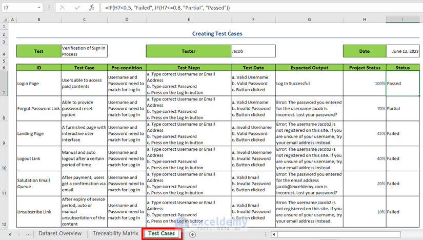
Regards
ExcelDemy
Hello Fortune,
In Your Products list you can add products of your choice. You will need to update the range according to your product list.
Regards
ExcelDemy
Hello Saqib Haroon,
In this article we used Excel’s stocks data to import stocks. Here is the list of Stocks financial data sources.
Saudi Arabia and Pakistan markets stock prices are not listed in Microsoft Excel stocks. You can use the Yahoo Finance API to get the stock prices if stocks are listed in there.
Regards
ExcelDemy
Hello,
You are most welcome. Thanks for your appreciation. Glad to hear that the article’s step by step explanations is helpful to you. Keep learning Excel with ExcelDemy!
Regards
ExcelDemy
Hello Mostain,
You are most welcome and thank you for your kind words! We will definitely consider creating a tutorial on this. Meanwhile, a VBA solution would work well for your needs.
Here’s a VBA solution to search through a closed workbook, retrieve matching rows from all sheets, and paste them into the active workbook without case sensitivity:
This code prompts for a search term, opens a closed workbook, finds the value across all sheets (ignoring case sensitivity), and copies the entire row to the last row of the active workbook. Simply update the workbook path, and it should work perfectly for your needs!
Regards
ExcelDemy
Hello,
You are most welcome. Thanks for your appreciation. Glad to hear that the article’s step by step explanations is helpful to you. Keep learning Excel with ExcelDemy!
Regards
ExcelDemy
Hello Lili,
You are most welcome. You can adapt Method 1 from this article on sending emails based on dates. Here’s an updated VBA code snippet that checks if the date in column B matches today’s date before sending the email.
This code will check the date in column B and send the email if the date matches today’s date.
Regards
ExcelDemy
Hello Liliana,
You are most welcome. You can adapt Method 1 from this article on sending emails based on dates. Here’s an updated VBA code snippet that checks if the date in column B matches today’s date before sending the email.
This code will check the date in column B and send the email if the date matches today’s date.
Regards
ExcelDemy
Hello Lucie,
You are most welcome. Glad you found the guide helpful! Regarding the error with union(body(‘Select’),body(‘Select’)), it’s possible the issue might be with the apostrophes. Make sure you’re using straight quotes (‘) instead of curly ones (‘ or ’). Additionally, double-check that both body(‘Select’) expressions reference valid and correctly named outputs.
If everything looks correct and the issue persists, feel free to share more details. I’d be happy to help troubleshoot further!
Regards
ExcelDemy
Hello Ian Lavell,
You are most welcome. Thank you so much for your feedback! I’m glad the explanation helped, and no worries at all about being a “slow learner”. We all have our own pace, and it’s great that you’re exploring VBA!
You’re absolutely right about applying the same logic to CommandButtons. The code you’ve shared looks great, and it’s fantastic that you’re combining the button caption with the ComboBox values to set the date.
Keep up the great work! Feel free to ask if you need any further clarifications.
Regards
ExcelDemy
Hello Tomasz,
You are most welcome. Glad to hear that you found the expected solution. Thanks for your appreciation and feedback. Keep learning Excel with ExcelDemy!
Regards
ExcelDemy
Hello Simon Gray,
You are most welcome. Glad to hear that the solution worked. Thanks for your appreciation and feedback. Keep learning Excel with ExcelDemy!
Regards
ExcelDemy
Hello Lethabo Mokoti,
You are most welcome. Keep learning Excel with ExcelDemy!
Regards
ExcelDemy
Hello Ian Lavell
You are most welcome and thank you for following along! The “Compile Error: Variable not defined” on i likely occurs because the variable i hasn’t been declared.
Try adding Dim i As Integer at the beginning of your code, before the For i = 1 to 41 line. This declares i as an integer, ensuring it’s recognized in the loop. Also, ensure that the rest of the subroutine is correctly typed, and the range/variables are properly referenced.
Regards
ExcelDemy
Hello Simon,
You are most welcome. Thanks for your appreciation and feedback. To hardcode the ranges and remove the input boxes from the script, you can directly assign the ranges in the code. Replace the lines where Application.InputBox is used with specific references like this.
To stop auto-adjusting row widths when pasting, remove the Columns.AutoFit line.
Regards
ExcelDemy
Hello Paul,
Each line of the email body starts and ends with vbNewLine for formatting. The _ at the end of each line allows you to split longer lines across multiple lines for readability. You can follow this breakdown to understand how each line flows.
Regards
ExcelDemy
Hello,
You are most welcome. Thanks for your insightful feedback. Keep learning Excel with ExcelDemy!
Regards
ExcelDemy
Hello Erika Póta,
Thanks for your input! While your method works perfectly, our original approach isn’t wrong. It just serves a different purpose by allowing for flexibility with additional color formats. Your simplified version works well and avoids the error. However, the Select Case structure could still be useful if more color options or formats are needed in future modifications. I appreciate your solution for directly calculating the RGB values.
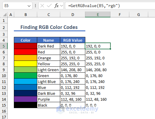
Our solution is working fine:
Regards
ExcelDemy
Hello,
You are most welcome. Thanks for your appreciation. Glad to hear that you found the examples clear and insightful. Keep exploring Excel with ExcelDemy!
Regards
ExcelDemy
Hello,
You are most welcome. Thanks for your appreciation. Glad to hear that these shortcuts is saving your time while working in Excel. Keep exploring Excel with ExcelDemy!
Regards
ExcelDemy
Hello Van Weaver,
You are most welcome. Glad to hear that you got your desired result. Keep exploring Excel with ExcelDemy!
Regards
ExcelDemy
Hello,
You are most welcome. Thanks for your appreciation. Glad to hear that the examples are helpful to you. Keep learning Excel with ExcelDemy!
Regards
ExcelDemy
Hello,
Thanks for your appreciation. Glad to hear that our Excel template is helpful to you. Keep learning Excel with ExcelDemy!
Regards
ExcelDemy
Hello George Shawnessey,
It looks like the issue comes from the syntax of the Application.OnKey method. To make F12 act as the “Break” key, unfortunately, you cannot use {Break} as an argument directly, as “Break” isn’t a valid key constant for OnKey. However, you can define a custom macro to handle a “break-like” functionality.
Here’s a suggestion:
Define F12 to trigger a macro:
Sub CreateBreakKey()
    Application.OnKey "{F12}", "BreakMacro" ' Assign F12 to trigger BreakMacro
End Sub

Sub BreakMacro()
    MsgBox "Break key activated!" ' Define your desired action here
End Sub
This setup triggers BreakMacro when F12 is pressed, allowing you to customize the “break” functionality.
Regards
ExcelDemy
Hello Van Weaver,
To sum a defined range of columns while still applying criteria for the rows, you can use the SUMPRODUCT function combined with INDEX and MATCH. For summing through a range of weeks up to today, consider using a dynamic approach.
1. Define the range for weeks in columns.
2. Use a dynamic condition like COLUMN()<=MATCH(TODAY(), your_week_range, 0) to sum only up to today.
3. Apply row criteria within the SUMPRODUCT for filtering.
Regards
ExcelDemy
Hello Sergio Zuniga,
To keep the original timestamps intact when filtering or sorting while still allowing updates when changes are made, you’ll need to modify the VBA code. Use a Worksheet_Change event to record the time only when a new entry is made or a change occurs, rather than recalculating the time every time the cell is referenced.
1. Right-click the sheet tab and choose View Code.
2. Insert this VBA code.
Private Sub Worksheet_Change(ByVal Target As Range)
    If Not Intersect(Target, Me.Range("B:B")) Is Nothing Then
        If Target.Cells.Count = 1 Then
            If Target.Value  "" Then
                If Me.Cells(Target.Row, "C").Value = "" Then
                    Me.Cells(Target.Row, "C").Value = Format(Now, "dd-mm-yy hh:mm:ss")
                End If
            Else
                Me.Cells(Target.Row, "C").ClearContents
            End If
        End If
    End If
End Sub
Time is recorded in column C when a value is entered in column B.
The timestamp won’t update during sorting or filtering.
If a value is changed manually, the timestamp will only update if the cell in column C is empty.
Regards
ExcelDemy
Hello Paul,
You can use this updated VBA code that will send an email when a cell in column F is >= 0 and include information from columns A and F in the email body.
Option Explicit
Dim Rng As Range

Sub Worksheet_Change(ByVal Target As Range)
    On Error Resume Next
    ' Check if more than one cell is changed
    If Target.Cells.Count > 1 Then Exit Sub

    ' Limit the range to A2:O48
    Set Rng = Intersect(Me.Range("A2:O48"), Target)
    If Rng Is Nothing Then Exit Sub

    ' Check if the cell in column F is >= 0
    If Not IsNumeric(Target.Value) Then Exit Sub
    If Target.Column = 6 And Target.Value >= 0 Then
        Call SendEmail(Target.Row)
    End If
End Sub

Sub SendEmail(rowNum As Long)
    Dim mApp As Object
    Dim mMail As Object
    Dim mMailBody As String
    Dim ws As Worksheet

    Set ws = ThisWorkbook.Sheets("2024 service") ' Change to your sheet name
    Set mApp = CreateObject("Outlook.Application")
    Set mMail = mApp.CreateItem(0)

    ' Prepare email body with info from column A and F
    mMailBody = "Hello," & vbNewLine & vbNewLine & _
                "Please note that item in row " & rowNum & " requires attention." & vbNewLine & _
                "A: " & ws.Cells(rowNum, 1).Value & vbNewLine & _
                "F: " & ws.Cells(rowNum, 6).Value & vbNewLine & _
                vbNewLine & "Regards," & vbNewLine & "Outlet Team"

    ' Send email
    On Error Resume Next
    With mMail
        .To = "[email protected]" ' Change to recipient’s email
        .Subject = "Alert: Cell in Column F >= 0"
        .Body = mMailBody
        .Display ' or you can use .Send to send the email directly
    End With
    On Error GoTo 0
    ' Clean up
    Set mMail = Nothing
    Set mApp = Nothing
End Sub
Worksheet_Change Event triggers when any cell in the range A2 changes. Sends an email when a cell in column F is greater than or equal to 0. Includes the information from columns A and F for the corresponding row in the email body.
Regards
ExcelDemy
Hello,
You are most welcome. Glad to hear that you found the article helpful. Keep exploring Excel with ExcelDemy!
Regards
ExcelDemy
Hello,
You are most welcome. Glad to hear that you found the article helpful. Keep exploring Excel with ExcelDemy!
Regards
ExcelDemy
Hello Paul,
You are most welcome. It looks like there are a couple of issues in your VBA code that need fixing:
1. The range check should specifically look at column F only.
2. You need to correct the index for the columns A and E in the email body.
The code now checks only column F (F2) for red cells.
Corrected the indices for columns A and E (1 for A, 5 for E).
Regards
ExcelDemy
Hello Monika Salinas,
It seems like you’re facing a common issue with links to external workbooks in Excel.
If your links stop working after the first click, it might be due to the linked workbook being closed or moved.
Make sure the file path remains valid and the linked workbook is open when you access it.
Additionally, check if there are any settings in Excel that might restrict external links.
Regards
ExcelDemy
Hello Roel,
To ensure your system automatically sends an email when the expiration date reaches 30 days, you need to adjust your VBA code slightly. The apostrophe before the .Send line is preventing the email from being sent. Removing that apostrophe will allow the email to be sent automatically.
Here’s how you can modify the SendEmail sub-procedure:
Make sure to replace “[email protected]” with your actual email address. Additionally, ensure that your main subroutine correctly checks for the conditions to trigger the email alert based on cell color changes.
If you follow these steps, you should receive automatic email notifications as intended.
Regards
ExcelDemy
Hello Roel,
To address your first concern about receiving multiple emails due to the same expiration date, you can modify the code to ensure only one email is sent per unique expiration date. This can be done by adding a simple check to track which dates have already triggered an email. Here’s how you can adjust the code:
This update ensures that for any particular expiration date, only one email will be sent.
Regards
ExcelDemy
Hello Bleona,
You can fix the runtime error 6 overflow by handling the large dataset more efficiently. Since you have over 1 million rows, Excel may be exceeding its memory limits. You can follow these steps:
1. Use smaller data batches for processing.
2. Switch from Integer to Long data types in your VBA code, as Integer can only handle values up to 32,767.
3. Consider using Power Query for merging large datasets instead of VBA, as it handles large data better.
Regards
ExcelDemy
Hello Leonardo,
The issue you’re encountering with VLOOKUP returning the incorrect time (e.g., 8:00 returning as 7:00) may be related to how Excel handles date and time values. Double-check that both columns are formatted exactly the same, not just visually but also in terms of underlying data types (i.e., as date/time values).
Sometimes even slight formatting differences or time zone offsets can cause such issues. You might also try using TEXT functions to standardize the format.
If VLOOKUP is fetching a time that’s off by an hour, consider verifying any regional settings or daylight saving time adjustments.
Regards
ExcelDemy
Hello Dear,
You are most welcome. Glad to hear that our article helped you to create relational database in Excel. Keep exploring Excel with ExcelDemy!
Regards
ExcelDemy
Hello Paul,
You are most welcome. To automate email notifications when a cell turns red, you can update your existing VBA code to check the cell color. You can use the Interior.Color property to identify red cells. Once a red cell is found, compile the data from that row and include it in the email body.
Sample VBA Code:
1. This code checks the specified range (A1) in Sheet1 for red cells. If a red cell is found, it compiles information from that row and sends an email.
2. Remember to update the Range, Sheet name, and recipient email address as needed.
3. Make sure to enable macros and allow programmatic access to Outlook.
Regards
ExcelDemy
Hello Dear,
Thanks for your appreciation. We are glad to hear that out step-by-step guide is helpful to you. You can use our guide to create a sales report. Keep learning Excel with ExcelDemy!
Regards
ExcelDemy
Hello Fiona,
To calculate the time difference across shifts that span multiple days, you’ll need to adjust your formula. Instead of just using the MOD function, you can directly subtract the end time from the start time while ensuring the dates are included.
For example, if your end time is in cell D2 and your start time is in cell C2, you can use:
=(D2 + IF(D2 < C2, 1, 0)) - C2 This formula adds 1 day if the end time is earlier than the start time. Regards ExcelDemy
Hello Raj,
To create a horizontal bar chart with a line combo in Excel,
1. First Insert a regular Bar chart by selecting your data.
2. Then, right-click on the data series you want to change to a line and choose Change Series Chart Type.
3. Select the Combo option, and then choose Line for the desired series.
4. Adjust the chart layout and format as needed.
Regards
ExcelDemy
Hello Muhammad Azhan,
To create a graph of kurtosis values in Excel, follow these steps:
1. Create a table with your values and corresponding labels.
2. Highlight the relevant cells.
3. Go to the Insert tab >> select the desired chart type (e.g., bar or line chart).
4. Use chart tools to add titles, labels, and adjust formatting as needed.
Regards
ExcelDemy
Hello Peter,
Thanks for your feedback and solution. Hopefully it would be useful for the users. That’s a clever approach! Using a concatenated string to identify empty rows while avoiding zeros is effective. After you locate those rows with “somestring0,” deleting them is straightforward. This method provides a great alternative when sorting or filtering isn’t an option.
Regards
ExcelDemy
Hello,
You are most welcome. Thanks for your appreciation. Glad to hear that our functions breakdown helped you to understand the function arguments. keep learning Excel with ExcelDemy!
Regards
ExcelDemy
Hello Kevin Slabbert,
To right-align values in a data table in Excel charts, you’ll need to adjust the alignment of the data in the worksheet itself.
Go to the Home tab >> select Align Right.
Unfortunately, Excel doesn’t offer direct control over alignment within the chart’s data table, so the workaround is to format the source data in the worksheet. This change will reflect in the data table of the chart.
Regards
ExcelDemy
Hello,
You are most welcome. Thanks for your appreciation. Glad to hear our step-by-step guide is helpful to you. Keep learning Excel with ExcelDemy!
Regards
ExcelDemy
Hello Ian,
Thank you for your feedback! Unfortunately, Excel doesn’t allow direct editing of ranges with relative addressing. Your suggested approach of creating a new named range and updating references seems to be the best workaround. Another option could be to use a formula in the new range to pull in data from the existing named range while expanding it. This way, you can keep your original named range intact for reference.
To create a new named range that expands on an existing one, you can use the INDEX function combined with OFFSET. Example formula:
=OFFSET(NamedRangeStart, 0, 0, ROWS(NamedRangeStart), COLUMNS(NamedRangeStart) + AdditionalColumns)
Replace NamedRangeStart with your existing named range, and AdditionalColumns with the number of extra columns you want to include. This formula effectively creates a dynamic range that expands based on your specifications.
Regards
ExcelDemy
Hello,
You are most welcome. Thanks for your appreciation. Glad to hear that our tutorial helped you to remove carriage returns. Keep learning Excel with ExcelDemy!
Regards
ExcelDemy
Hello Ano Victory,
I’m glad you found it interesting! To force related selections when the first selection is changed (e.g., Fish/Salmon -> Fruit/Salmon), you could use dependent data validation. This way, the second selection will reset or limit options based on the first choice. You’ll need to set up a named range for each category and then apply data validation rules for the second dropdown accordingly.
You can use a Custom Data Validation with an IF statement to restrict invalid subcategory selections. For example, let’s say “Fish” is selected in the first dropdown, and you want to force the user to only choose “Salmon” or “Tuna” in the second dropdown. You can apply a formula like this in the second dropdown:
=IF(E1=”Fish”,OR(F1=”Salmon”,F1=”Tuna”),OR(F1=”Apple”,F1=”Orange”))
This will ensure that the second selection matches the first dropdown category.
You can adjust this formula based on your category-subcategory structure.
Regards
ExcelDemy
Hello Jay,
You are most welcome and thank you for your kind words! To change the individual segment colors for just one month, follow these steps:
1. Select the chart.
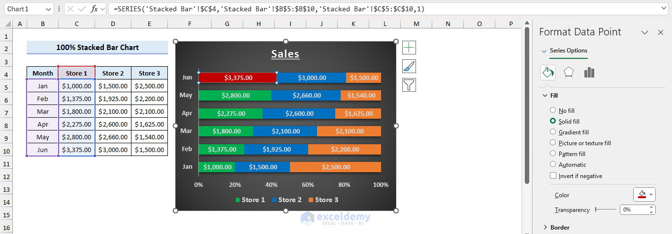
2. Select the bar segment for January that you want to modify.
3. Right-click the segment and choose Format Data Point.
4. In the Format Pane, change the Fill color to your desired choice.
Regards
ExcelDemy
Hello Shubham,
You can download the stock data like yahoo finance. Use the STOCKHISTORY function. Follow this article to get the stock prices with your required fields.
Download Historical Stock Data into Excel (with Easy Steps)
Regards
ExcelDemy
Hello,
You are most welcome. Thanks for your appreciation. Glad to hear that our step by step guide helped you to follow the instructions easily. Learn Excel with ExcelDemy!
Regards
ExcelDemy
Hello Joshua Goodman,
The spill error you’re experiencing could be due to extra data being included in your formula’s output. Please do the followings:
Ensure your formula only returns the employee data without repeating the department column.
You can use FILTER in combination with UNIQUE or INDEX to target just the employees.
Make sure the dragged formula doesn’t overlap the department list, which might trigger the spill error.
Feel free to share your formula with dataset for further investigation.
Regards
ExcelDemy
Hello,
You are most welcome. Glad to hear that our tutorial is lifesaver to you. Thanks for your appreciation. Keep learning Excel with ExcelDemy!
Regards
ExcelDemy
Hello Ron,
You are most welcome. Glad to hear that method 2 worked for you. Thanks for your appreciation. Keep learning Excel with ExcelDemy!
Regards
ExcelDemy
Hello Denise Groves,
You are most welcome. Glad to hear that our tutorial helped you to visualize nesting substitute formulas. Keep exploring Excel formulas with ExcelDemy!
Regards
ExcelDemy
Hello JaneM,
“Subscript Out of Range Error” occurs when trying to reference a worksheet that does not exist. In your case, ensure that the names of the sheets you are trying to access match exactly with what is in the workbook. To solve this issue you can use the following VBA code.
The code will dynamically checks for the existence of the sheets Sheet1(2) to Sheet1(11) using a loop. It will copy the entire rows based on the last used row in each sheet instead of using UsedRange, which may cause issues if you have formatting or other non-data cells.
The code creates a single new worksheet named MergedData and does not insert any blank sheets.
Copy-Paste the VBA code:
Regards
ExcelDemy
Hello Matthew Senko,
It seems that you’re encountering a syntax error in your Power Automate flow. The issue is likely related to how the date is formatted in your query. Make sure that the date is enclosed in double quotes and use the correct format.
Instead of: Deadline eq ‘2024-10-03’
Try using: Deadline eq ‘2024-10-03T00:00:00Z’
If the issue persists, please double-check your query syntax. Let me know if you need further assistance!
Regards
ExcelDemy
Hello Jim,
Thanks for the update! If you’re still encountering issues with Week 1, consider using the ISOWEEKNUM function to get the correct ISO week number:
=ISOWEEKNUM(A1)
This function aligns with your region’s definition of Week 1.
To account for ISO week numbering where Week 1 starts on the first week with at least four days, you can use the following formula:
=DATE(B5,1,4) – WEEKDAY(DATE(B5,1,4), 2) + (A5-1)*7
This should help correct the offset.
N.B: Leap years shouldn’t shift by a full week, but they could affect the day counts.
Regards
ExcelDemy
Hello Charlie,
To create a radar chart with 6 different scales, you can apply the same method shown in the article for multiple scales. Each axis in a radar chart can represent a separate scale.
You just need to ensure that your data is set up accordingly with six distinct series and adjust the axis limits for each. If you need help with a specific part of the process, feel free to ask!
Regards
ExcelDemy
Hello Laurie,
Here, oFolder object not being correctly initialized within the Do While Coll_queue.Count > 0 loop. That’s why the error is occurring. This object is necessary to iterate through files and subfolders, but it’s missing an assignment before looping over subfolders and files.
To fix this issue, assigning oFolder from the collection at the beginning of the loop.
This ensures oFolder is properly initialized and recognized when iterating over its subfolders and files.
Updated Excel File:
List All Files in Folders & SubFolders Including File Details with Excel VBA.xlsm
Regards
ExcelDemy
Hello Eduardo,
De nada! You are most welcome. Keep learning Excel with ExcelDemy!
Regards
ExcelDemy
Hello kellyd,
To solve your issue, you can use the INDEX and MATCH functions along with a filter to look up the first non-blank status for each site code.
In the “Status Lookup” column, use this formula:
=INDEX($C$15:$C$23,MATCH(1,($B15=$B$15:$B$23)*($C$15:$C$23<>“”),0))
After entering this formula, press Ctrl+Shift+Enter (if you’re not using Excel 365) to treat it as an array formula.
This will return the first non-blank status for each site code.
Regards
ExcelDemy
Hello Moegamat Shakier Stuurman,
You are most welcome. Thanks for your appreciation. Glad to hear that you are going to use it to track aging analysis. Keep exploring Excel with ExcelDemy!
Regards
ExcelDemy
Hello Raj,
Thanks for your appreciation. Keep exploring Excel with ExcelDemy!
Regards
ExcelDemy
Hello Minhaj,
In the formula =INDEX($B$140:$B$144,MATCH($C$146,$C$140:$C$144,1)+1), the +1 is used to return the value from the next row after the matched value.
Formula Explanation:
MATCH($C$146,$C$140:$C$144,1): This part searches for the value in cell C146 (which contains “Today’s Date”) within the range C140:C144 (the list of birthdays). The 1 at the end of the MATCH function indicates that the function looks for the largest value that is less than or equal to C146. So, it will return the position of the latest birthday before or on the current date.
+1: After the MATCH function finds the closest previous birthday, the +1 moves the selection to the next row in the range, which corresponds to the next upcoming birthday.
INDEX($B$140:$B$144,…): This part retrieves the name of the person who has the next upcoming birthday based on the MATCH result (which is adjusted by +1 to move to the next entry).
Regards
ExcelDemy
Hello Steve,
You can address the error by ensuring there is enough space in the target worksheet for the CSV data to be imported without overlapping existing tables or XML mappings. Consider moving the existing table to another location or importing the CSV data into a new worksheet and then linking it to the existing formulas or tables.
Regards
ExcelDemy
Hello,
You are most welcome. Thanks for your appreciation. Glad to hear that our examples helped you.
Regards
ExcelDemy
Hello,
You are most welcome. Thanks for your appreciation. Glad to hear that our examples helped you.
Regards
ExcelDemy
Hello Louis,
Thanks for your appreciation. Keep exploring Excel with ExcelDemy!
Regards
ExcelDemy
Hello Steve,
It’s clear you’re facing performance bottlenecks with Excel, and your frustration is understandable given your powerful hardware. Excel, while widely used, doesn’t fully utilize multi-core CPUs or GPUs for many tasks. Here are some steps and alternatives you could try:
To optimize Excel usage you can disable volatile functions like NOW() and RAND() recalculate constantly, slowing Excel down.
Overuse Conditional Formatting can heavily impact performance, especially on large datasets.
Set Excel to manual calculations when working on large datasets.
Excel doesn’t effectively leverage GPUs or advanced multi-threading. However, you can check File > Options > Advanced > Enable hardware graphics acceleration (though this often doesn’t make significant differences in complex datasets).
Try to enable multithreading by going to File > Options > Advanced > Formulas > Enable multi-threaded calculation. While Excel doesn’t scale well across many cores, this can still help somewhat with certain tasks.
Explore Alternatives:
Power BI: It’s optimized for large datasets and leverages more powerful backend engines for data processing.
Python (Pandas/NumPy): If you handle large matrix-like data, Python libraries can offer much faster performance and can use multiple cores efficiently.
R or SQL-based tools: These are better at handling larger datasets, parallel processing, and complex operations.
Consider Excel Online: While Excel desktop has limitations, Excel Online, backed by Microsoft’s cloud, sometimes offers better performance in dealing with larger datasets since it uses cloud resources.
Despite its strengths, Excel’s legacy architecture doesn’t yet match the potential of modern hardware. Exploring these steps or alternative tools might improve your workflow and reduce frustration.
Regards
ExcelDemy
Hello Hans Hallebeek,
It’s great to hear that you love to play with VBA. VBA is interesting. Here’s a sample code to handle an ActiveX TextBox Change event in a worksheet:
1. Insert an ActiveX TextBox from the Developer tab.
2. Open the VBA editor (Alt + F11).
3. In the Project Explorer, find the worksheet with the TextBox.
4. Now, write the following code in the worksheet’s code window:
This triggers a message box whenever the TextBox content changes. You can replace TextBox1 with your TextBox’s name.
Regards
ExcelDemy
Hello Timothy,
It seems the issue is due to the protection on the data sheets preventing your mainSht from accessing the necessary data. You can modify your VBA to temporarily unprotect the sheets when running the code.
You can also try setting the UserInterfaceOnly property when protecting the sheets. This allows VBA code to modify protected sheets while still restricting user interaction:
This way, your VBA code can still manipulate the data without fully unprotecting the sheets each time. I hope this helps! Let me know if you need further clarification or additional resources.”
This approach ensures the sheets remain protected for users but accessible for the code execution.
Regards
ExcelDemy
Hello Angufibo David,
Thank you so much for your kind words! I’m glad you found the material helpful. We’re always working to provide more detailed and practical examples, especially with Excel and VBA. If you have any specific topics you’d like to see covered, feel free to share!
Regards
ExcelDemy
Hello,
You are most welcome. Thanks for your kind words. Glad to hear that the invoice format is helpful to you. Keep learning Excel with ExcelDemy!
Regards
ExcelDemy
Hello,
You are most welcome. Thanks for your kind words. Glad to hear that the registry edit solution worked perfectly for you. Keep learning Excel with ExcelDemy!
Regards
ExcelDemy
Hello AT William,
You are most welcome. Thanks for your kind words. Keep exploring Excel with ExcelDemy!
Regards
ExcelDemy
Hello Edward M,
You are most welcome. Thanks for your appreciation. Glad to hear that it is helpful to you. Keep learning Excel with ExcelDemy!
Regards
ExcelDemy
Hello Edward M,
You can definitely modify the formula to reference a date in another cell instead of hardcoding it. For example, if you have a date in cell A1, you can use the formula =COUNTIF(E5:E27,”>” & A1) to make it dynamic. This way, you won’t have to change the formula every time you need a different date range.
Regards
ExcelDemy
Hello Roy E. McCarthy,
We are using MS Office 365. In Excel, once you freeze any row or column, the option will change to “Unfreeze Panes” instead of showing “Freeze Panes” again. This helps users know that something is already frozen. If you want to freeze or unfreeze rows or columns, you need to select the appropriate option based on your current status.
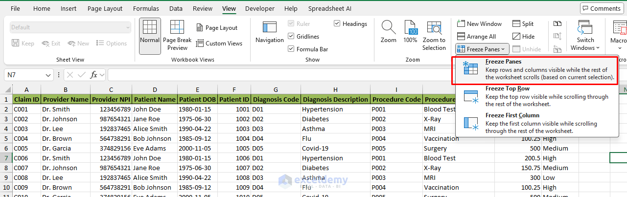
Before freezing anything:
After freezing first row:
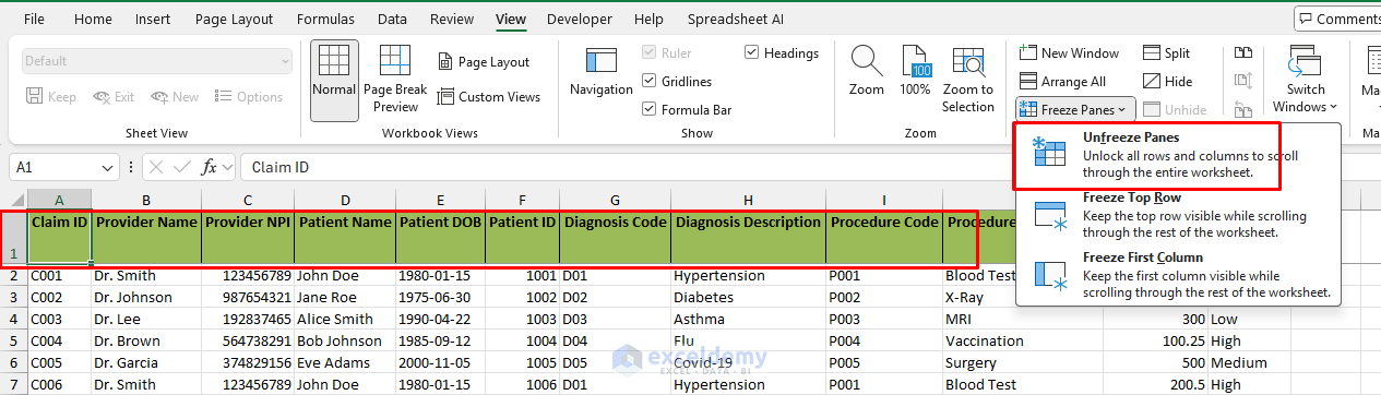
Regards
ExcelDemy
Hello Maddie,
It seems the custom number format you’re using might be interacting with the display unit settings in Excel.
Set the display units to “None”. Display units in Excel (e.g., “Thousands”, “Millions”) automatically append prefixes like “K” or “M”, and in this case, that’s why the “K” is appearing.
Use this custom format: 0.00,, “GW” or #.##,,”GW”
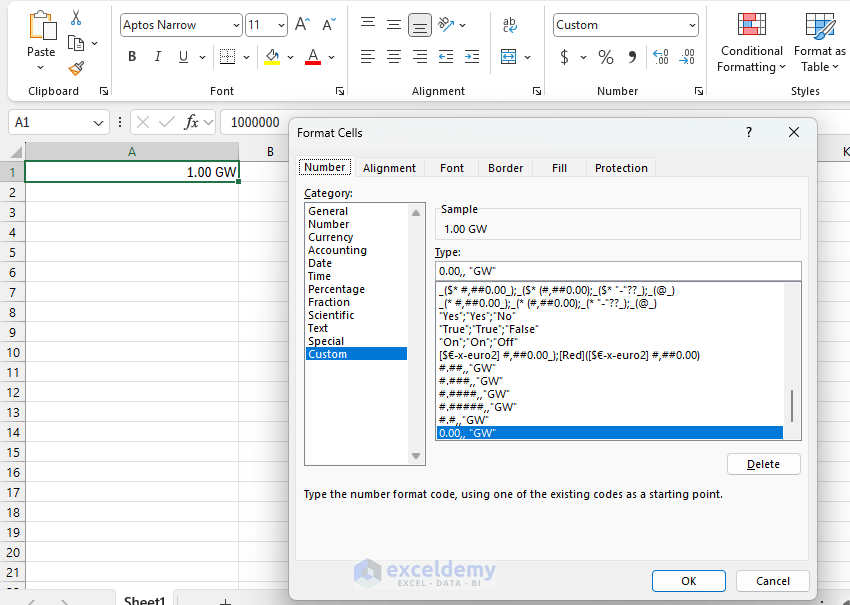
The double commas ,, divide the number by 1,000 twice, which effectively formats the number in thousands. The result should display values in thousands with “GW” as the unit but without adding “K”.
By setting the display units to “None” and using the format above, the unwanted “K” should no longer appear, and the values will remain visible.
Regards
ExcelDemy
Hello Grace,
It is possible to connect a spin button with a print button. The spin button can adjust the quantity of labels from the next sheet, and the print button can trigger printing based on the value selected. You would need to use a combination of VBA code to link the spin button’s value to the print process, specifying the number of copies using the spin button control.
First, insert the Spin Button and assign it a cell for its value (e.g., Sheet1!A1).
Then, add the Print Button and assign the following VBA code:
This code reads the quantity from the spin button and prints the label sheet that many times.
Regards
ExcelDemy
Hello Maddie,
To display units in thousands without “K”. You can use the format #.##,,”GW” for thousands (without “K”).
This removes the extra “K” while formatting the number in thousands.
Regards
ExcelDemy
Hello Shan,
To dynamically feed cell addresses from an Excel file (starting at cell B3), you can modify the VBA code to read the list directly from that file.
This will read the cell addresses from column B of the other file and highlights them in the current workbook. Remember to replace “ChangesFile.xlsx” with the actual name of your file.
Regards
ExcelDemy
Hello Shan,
Glad to hear. To dynamically feed cell addresses from an Excel file (starting at cell B3), you can modify the VBA code to read the list directly from that file.
This will read the cell addresses from column B of the other file and highlights them in the current workbook. Remember to replace “ChangesFile.xlsx” with the actual name of your file.
Regards
ExcelDemy
Hello,
You are most welcome. Thanks for your appreciation. Glad to hear that you will apply the examples in your project. Keep learning Excel with ExcelDemy!
Regards
ExcelDemy
Hello Shan,
To highlight the range with changes, you’ll need to use VBA to highlight the changed cells in the original Excel file.
If the compare tool generates a range like (A101, B95, etc.). You’ll need to copy this list.
Open the workbook where changes occurred. Then, run the following VBA script to loop through the list and highlight the cells.
It will highlight the specified cells with a yellow background.
Regards
ExcelDemy
Hello Doreen Bagola,
The formula we used to calculate annual leave can be adjusted for leave donations and administrative leave, but you’ll likely need to customize it depending on how these types of leaves are tracked.
For instance, you can add extra columns or rules to include donated or administrative leave alongside the regular annual leave calculations. This will ensure all leave types are accounted for. You may need to adjust data validation or leave balance formulas accordingly.
Regards
ExcelDemy
Hello Gail Anthony,
Yes, it is possible for a cell to reference its own sheet name in Excel. You can use a formula like this:
=MID(CELL(“filename”, A1), FIND(“]”, CELL(“filename”, A1)) + 1, 255)
This formula extracts the sheet name from the full file path returned by the CELL(“filename”, A1) function. Just ensure the workbook is saved, as the filename includes the sheet reference.
Regards
ExcelDemy
Hello,
You are most welcome. Glad to hear that our tips are helpful to you. Keep exploring Excel with ExcelDemy!
Regards
ExcelDemy
Hello بهروز مظفری,
To merge all data from different sheets to one single workbook. You can follow the step by step guide of these articles:
How to Combine Multiple Worksheets into One Workbook?
How to Merge Sheets in Excel – Must-Know Tips and Techniques
How to Merge Multiple Sheets into One Sheet with VBA in Excel?
Regards
ExcelDemy
Hello Jeremy,
You are most welcome. Thanks for your appreciation. To calculate the elapsed time between two date-time entries in Excel, you can subtract the two cells and display the result in decimal hours. But you must need to use the date and time format properly. You can’t use colon(:) in between date and time.
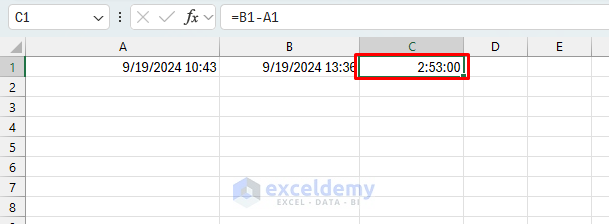
Use this formula to subtract G21 from G22:
=G22 – G21
Format the result cell as [h]:mm:ss.
Select the cell T21 >> Right-click >> select Format Cells >> select Custom >> type [h]:mm:ss
Multiply the result by 24 to get the answer in hours:
=(G22 – G21) * 24
Excel naturally handles dates and times. When subtracting times that span over midnight, the same formula will work.
Regards
ExcelDemy
Hello Suzanna Cocker,
You are most welcome. Thanks for your appreciation. To remove the pictures added via VBA, you can create another macro assigned to a button to delete them. Copy paste the VBA code that will remove all the shapes (including images) from the sheet.
This code will delete all pictures in the active sheet when the button is clicked. You can add this to your existing setup.
Regards
ExcelDemy
Hello Ravi Patel,
To ensure that images match the corresponding name in column A, you can compare the image name with the text in column A (e.g., abc in column A should match abc.jpg), and then insert that image into column B.
In the original code, it opens a dialog box to select multiple images, and then it adds them one by one in adjacent cells. If the image names don’t match, you would need to adapt this logic based on image names stored in column A. To automate the matching with your scenario, make sure the file names match the corresponding data in column A.
Regards
ExcelDemy
Hello Sophie,
To automatically moves a row when the status is marked as “done”. You can use the Worksheet_Change event along with the existing code for moving rows.
This will check the changes in the “Status” column (Column C in this case). If the status changes to “done”, the MoveRow_DeleteOriginal subroutine is triggered. You can modify the range and the condition (Target.Value = “done”) as needed for your specific use case.
Regards
ExcelDemy
Hello Fin,
The “-2” or “-3” are the different adjustments for kurtosis calculations. In this article, “-2” is used in the context of excess kurtosis, which helps measure how heavy or light-tailed the distribution is compared to a normal distribution.
Normally, kurtosis is 3 for a normal distribution. Some methods subtract 3 from kurtosis (excess kurtosis), while in other cases, adjustments like “-2” are made based on specific analysis needs. It’s essential to know which method or software you’re using.
Regards
ExcelDemy
Hello Kevin,
Thanks for your solution. Hope it will be helpful for our Excel users. Thanks for contributing. Let’s explore Excel with ExcelDemy!
Regards
ExcelDemy
Hello Frank,
Thanks for your suggestion. It’s the beauty of Excel it provides better formula with updated functions. FILTER function is one of the most dynamic and useful function. Keep contributing Excel tips with ExcelDemy!
Regards
ExcelDemy
Hello,
You are most welcome. Thanks for your appreciation it means a lot to us. We focus on the formula explanation too. Keep exploring Excel with ExcelDemy!
Regards
ExcelDemy
Hello Esther,
You are most welcome. Thanks for your appreciation it means a lot to us. Keep exploring Excel with ExcelDemy!
Regards
ExcelDemy
Hello Nguyen,
You are most welcome. It’s okay don’t feel sorry. Keep exploring Excel with ExcelDemy!
Regards
ExcelDemy
Hello Sanjay Dutt Dobhal,
To calculate the time difference you need to insert the date and time based on your regional settings of Excel.
Format the date and time based on your settings then use the CONCATENATE formula to calculate the time difference from date and time.
=CONCATENATE(C2,””,D2)-CONCATENATE(A2,””,B2)
Right-click the time difference cell >> choose “Format Cells” >> select “Custom” and enter the format [h]:mm
Regards
ExcelDemy
Hello Emz,
The purpose of computing or finding the running total in a pivot table is to observe cumulative values over time or sequential categories. It will help you to identify trends, monitor progress, and understand how data accumulates.
For example, in sales data, a running total allows you to see how much revenue has been generated up to a certain point. It provides insights into overall performance, allowing for easier analysis of growth or decline. This is especially useful in tracking inventory, financial data, or project timelines.
Regards
ExcelDemy
Hello AML,
You can add IF statement to adjust font color based on background brightness in the VBA code. You can add a condition that sets the font color to white for darker backgrounds and black for lighter ones.
Condition to add lighter color on a darker background and vice-versa:
Place this inside the loop where you’re setting background colors. This will ensure visibility based on the background color.
Regards
ExcelDemy
Hello Jacquelyn Luna,
To save stopwatch times into a column in the same spreadsheet, you can modify the VBA code in Excel. You will need to modify the StopTimer() subroutine to save the stopwatch times into a column in Excel.
First, go to the module and update the code of Stop button.
Add the following code to save the time into the next available row in a specific column:
The lastRow variable finds the next empty row in column A. Sheets(“Sheet1”).Cells(lastRow, 1).Value = Range(“B4”).Value saves the current stopwatch time from cell B4 into column A.
This will store each time result when you stop the timer. Adjust the sheet and cell references as needed for your workbook.
Regards
ExcelDemy
Hello Amy,
You can try using a combination of SEARCH and INDEX-MATCH.
In cell U2 on Tab 1, try the following formula:
=IFERROR(INDEX(‘Tab 2’!B:B, MATCH(TRUE, ISNUMBER(SEARCH(‘Tab 2’!A:A, T2)), 0)), “”)
1. SEARCH(‘Tab 2’!A:A, T2) checks if any value from column A on Tab 2 is found in the text in column T on Tab 1.
2. INDEX(‘Tab 2’!B:B, …) returns the corresponding value from column B on Tab 2.
3. IFERROR handles cases where no match is found.
This should return the desired result in column U of Tab 1.
Regards
ExcelDemy
Hi Akhila,
You are most welcome. Thank you for your comment! We provide sample datasets to help you get started, and you can easily extend or modify them as needed. Feel free to add more rows to suit your specific use case or dataset requirements. The sample data we’ve provided is designed to be a foundation for building your own healthcare insurance claim datasets.
Regards
ExcelDemy
Hello Akhila,
Here is the sample dataset of Healthcare Insurance Claim Patients
Download the Dataset: Healthcare-Insurance-Claim-Patients-Dataset.xlsx
Regards
ExcelDemy
Hello Adnan,
You are most welcome. Thanks for your appreciation. The “50” and “100” columns represent performance benchmarks. The “50” column typically indicates a baseline or minimum acceptable performance, while the “100” column represents the ideal or target performance level. The “Actual” column shows the real performance values. The “Score” column reflects how close the actual performance is to these benchmarks, and it is multiplied by the corresponding weight to calculate the “Weighted Score.” The total weighted scores are summed to determine overall performance (82 in this case).
Regards
ExcelDemy
Hello Ken Mambo,
You are most welcome. To add a cumulative totals table for days present or absent using the article’s attendance sheet, you can follow these steps:
Add a table with rows representing months and columns for each employee.
In the cumulative table, for each month use:
=COUNTIF(Range_of_Attendance, “P”) // For Present Days
=COUNTIF(Range_of_Attendance, “A”) // For Absent Days
For cumulative data, use:
=SUM(January_Cell:Current_Month_Cell)
This approach will give you cumulative totals month by month.
Regards
ExcelDemy
Hello Dan,
Gmail doesn’t natively allow sending emails via VBA due to security restrictions. However, you can try to send emails via Gmail by using CDO (Collaboration Data Objects) with SMTP.
Google may block this unless you’ve allowed less secure apps or set up an app-specific password if you’re using two-factor authentication (2FA).
For Google Sheets, using Google Apps Script would be more appropriate since it integrates seamlessly with Gmail. Here’s how you can approach both:
Apps Script is directly integrated with Google’s ecosystem, making it an easier option for automating email alerts, and it’s more secure than trying to bypass restrictions in Gmail for VBA.
Regards
ExcelDemy
Hello Aisling,
Thanks for your appreciation. To add more interests you’ll need to extend the interest rate list manually and adjust the formulas to include the new entries.
Here’s how to do it:
1. Add the additional 10 interest rates (or however many you need) in the interest rate table.
2. Modify any formulas that reference the original range to accommodate the extended list.
If you’re facing difficulties, ensure all formulas reflect the new range.
Regards
ExcelDemy
Hello,
In our Excel file the code is working perfectly without errors.
The possible reasons of getting errors in you end might be: Selecting a range at the edge of the worksheet or having non-contiguous selections.
You can add a check to avoid out-of-bounds errors:
This prevents the code from trying to access an offset that doesn’t exist (the last row in the selection).
Regards
ExcelDemy
Hello Kelly,
To extend the Highlight Active Row functionality outside a table, you can apply Conditional Formatting using a formula. Here’s how:
1. Select the entire range (or the rows you want to highlight).
2. Go to Home > Conditional Formatting > New Rule.
3. Choose “Use a formula to determine which cells to format.”
4. Enter the formula: =ROW()=CELL(“row”)
5. Select your preferred format.
This will highlight the active row across the selected range, even outside of tables.
Regards
ExcelDemy
Hello Franck,
You are most welcome. Since you don’t have Office 365, you can try using Google Sheets with the GOOGLEFINANCE function to import financial data for free, or explore third-party APIs like Alpha Vantage. These are good alternatives to the STOCKHISTORY function in Excel.
Regards
ExcelDemy
Hello Y2mateOfficial,
You are most welcome. Glad to hear that you found our template super helpful. Our calculator helps to calculate my bank interest efficiently. Keep learning Excel with ExcelDemy!
Regards
ExcelDemy
Hello Shimmy,
You are most welcome. Glad to hear that you found our article helpful. Keep learning Excel with ExcelDemy!
Regards
ExcelDemy
Hello MP,
You are most welcome. Modified the VBA code by unprotecting the worksheet at the start of the macro and reprotecting it at the end.
Unprotects the worksheet when a selection is made. Reprotects it afterward using UserInterfaceOnly:=True, allowing macros to work while the sheet remains protected.
Make sure to replace “YourPassword” with your actual password and “YourRange” with the cell range that contains the drop-down list.
Regards
ExcelDemy
Hello DD,
You’re right. The method in the article works well for fixed text but doesn’t apply to dynamic text like formulas (=A1, etc.). In Excel, there isn’t a built-in feature to rotate text 180 degrees for cell references or formulas.
you can use a shape or text box, link the shape’s text to the formula (e.g., =A1), and then rotate the shape. While this doesn’t work directly inside a cell, it provides a solution for visualizing rotated dynamic text. It may not be ideal for every case but can help when dealing with variable data.
Regards
ExcelDemy
Hello Sathish,
To insert pictures horizontally across a row (e.g., A1, B1, C1…), changed the loop to increment the column index (PicColIndex) instead of the row index.
Here’s the updated code:
Regards
ExcelDemy
Hello Sathish,
To insert pictures horizontally across a row (e.g., A1, B1, C1…), changed the loop to increment the column index (PicColIndex) instead of the row index.
Here’s the updated code:
Regards
ExcelDemy
Hello Savoir-faire,
Thanks for pointing this out! Using OR with arrays can sometimes lead to unreliable results, especially in non-array formulas or older Excel versions. It’s better to use more robust methods like MATCH or COUNTIF, which handle list comparisons more efficiently and avoid edge cases where OR might fail. We used OR in this context is its simplicity and readability. For users working with Excel 365 or newer versions, this method provides an easy way to compare multiple values without needing complex functions like MATCH or COUNTIF. It’s particularly helpful for small datasets and straightforward checks. Additionally, the OR function works well for quick visual comparisons in smaller spreadsheets.
Regards
ExcelDemy
Hello HR,
If you want to input 0.5 as half day leave. You can use the following formula for Half Day (HD) column: =SUMPRODUCT(–($D9:$AH9=”HD”)*0.5)
It will look for all occurrences of “HD” within the range $D9:$AH9. Each “HD” will be counted as 0.5.
You will need to format the cells with 2 decimal places to properly show the decimal number otherwise it will show you rounded 1.
Regards
ExcelDemy
Hello Nafiu Gide,
There are functions that can arrange columns based on their date by rows. To combine sorting columns by dates and rearranging rows dynamically, you can use the SORT function along with INDEX to reference the sorted columns and match the data accordingly.
Formula:
=INDEX(A2:D5,,MATCH(SORT(A1:D1),A1:D1,0))
This formula sorts the dates in A1:D1 and aligns the data in A2:D5 accordingly.
Regards
ExcelDemy
Hello Calvet,
You are most welcome. Thanks for your appreciation. We are glad to her that you found our article helpful and informative. Keep learning Excel with ExcelDemy!
Regards
ExcelDemy
Hello Franck,
Yahoo Finance has recently changed its API access, leading to authentication failures for many users starting around September 6, 2024. Users are encountering errors such as “unauthorized” or “not found,” it seems that Yahoo has either restricted the free access to its data or implemented new authentication methods.
You can use the alternatives STOCKHISTORY function in Excel (for Office 365 users) or exploring paid options from Yahoo may be necessary.
Regards
ExcelDemy
Hello Azada Rudnicki,
We use Microsoft Excel 365 to demonstrate the examples. The reason of getting 0 is GET.CELL function is not working properly or not defined in the Name Manager. IF function works with existing values there is no problem in the formula.
Before using the IF formula you must need to create the name manager by using GET.CELL function.
Steps:
=GET.CELL(38,'Example 1'!B5)=CellColorRegards
ExcelDemy
Hello Terry,
To compare the total cost of a $500,000 mortgage with simple and compound interest (annual compounding) at 5% over 20 years, you can create a spreadsheet with two sections:
Simple Interest Formula: I=P*r*t
Use the formula =500000 * 5% * 20 to calculate the total interest for simple interest.
Compound Interest Formula: =500000 * (1 + 5%)^20 – 500000
In Excel: =FV(B2, B3, 0, -B1) – B1
Now calculate the differences and display them in a printout or spreadsheet.
Downlaod Excel File:
Mortgage-Interest-Comparison.xlsx
Regards
ExcelDemy
Hello Musthafa,
To prepare manual bin card you can follow the steps of our article,
1. Design a standard bin card with fields like Item Name, Item Code, Quantity, etc.
2. Ensure your item data is stored in a separate Excel worksheet with columns for Item Name, Code, Quantity, etc.
3. To automatically pull data from your stock worksheet to the bin card, use the VLOOKUP function (or INDEX-MATCH for more flexibility).
For example, if the item code is in cell A2 of your bin card, and your item data is in a worksheet named “StockList,” the formula to fetch the item name might look like this:
=VLOOKUP(A2, StockList!A2:E100, 2, FALSE)
This formula will search for the item code in column A of “StockList” and return the item name from column B.
You can use VBA code to automatically loops through each item in the stock list, populates the bin card template, and prints it. Ensure that your bin card is properly formatted for printing. You can do this by setting print areas and page breaks.
Run the VBA to automatically fill and print bin cards for all items in your stock.
Regards
ExcelDemy
Hello MP,
Glad to hear that all the VBA code is working perfectly. To address the issue where the multiple selection drop-down stops working after protecting the worksheet, you need to modify the VBA code to allow edits to the specific cells while keeping the rest of the sheet protected. You can use the UserInterfaceOnly:=True parameter when protecting the sheet, which allows macros to make changes while maintaining protection for users.
You can add UserInterfaceOnly:=True in the VBA code,
It will run without unprotecting the sheet. Add this code in the Workbook_Open event to ensure the protection is applied every time the workbook is opened. Provide “YourSheetName” and “YourPassword” accordingly.
Regards
ExcelDemy
Hello Weronika,
To change the calendar’s weekday order you will need to change the labels name and update the VBA code date filling logic.
To start with Monday and end with Sunday in the Excel date picker, change the order of the day labels (e.g., Label1.Caption = “Mon”, Label7.Caption = “Sun”).
Now, use the updated Create_Calender procedure. Changed the Weekday function to use vbMonday, ensuring that the week starts on Monday. and the rest of the logic remains the same to ensure proper date filling and formatting.
Download the Excel File:
Calendar-Date-Starts-with-Monday.xlsm
Regards
ExcelDemy
Hello Ahmed,
You are most welcome. Thanks for your appreciation it means a lot to us. Keep learning Excel with ExcelDemy!
Regards
ExcelDemy
Hello Don,
Thanks for your feedback! This article is written based on the Windows version of MS Office 365, where dynamic named ranges works across charts.
It seems Excel 2016 on Mac behaves differently, allowing only workbook-level named ranges and replacing worksheet references with the workbook name. Unfortunately, for existing charts, this dynamic range may not apply correctly, and creating new charts might be the only solution on Mac.
We appreciate your insight, and we’ll consider these differences in future content!
Regards
ExcelDemy
Hello Tigran,
You can use a combined formula to search with two tags in Excel. Use the SEARCH function for each tag and the AND or OR operators to meet your criteria.
Formula:
=AND(ISNUMBER(SEARCH(“Tag1”, A2)), ISNUMBER(SEARCH(“Tag2”, A2)))
This formula will return TRUE if both tags are found in the text, or FALSE otherwise. Based on your criteria and need you can adjust this formula tags and reference.
Regards
ExcelDemy
Hello Anne K,
You can modify the logic of calculating Normal hours (column N) and OT hours (column P), specifically targeting the total at the bottom of each column. If Normal hours (column N) is less than 38, then part of the OT hours (column P) should be added to reach 38. Once Normal hours reach 38, any remaining OT should stay in column P.
In the cell where you total your Normal hours (say N20), you can use this formula to adjust for the scenario where OT hours should be added to the Normal hours if the total normal hours are less than 38.
Updated Formula:
=MIN(38, SUM(N12:N19) + SUM(P12:P19))
In the cell where you total your OT hours (say P20), adjust the OT formula so that it only shows overtime that is truly above 38 hours of work.
Updated Formula:
=MAX(0, SUM(L12:L19) – 38)
This should solve the issue where overtime hours need to “make up” for missing normal hours but still allows for extra OT beyond 38 hours. Let me know if this works for you or if you need any further tweaks!
Regards
ExcelDemy
Hello Nick Throp,
The reason of the getting 438 error is you don’t have the on behalf permission. To set the “From” field in an email using VBA in Outlook, you must need to have “Send As” or “Send on Behalf” permissions for the generic email you want to use. Without these permissions, .From property will result in a 438 error.
To use .From property you should contact to IT admin to obtain the required permissions for the generic email address. Once permissions are granted, the VBA code should work without throwing an error.
Here’s an example of setting the “From” field:
MailItem.SentOnBehalfOfName = “[email protected]”
This approach will allow you to send emails on behalf of another account if you get the permission.
Regards
ExcelDemy
Hello HC,
Thank you for your comment! The confusion arises from auto-rounding the numbers (not showing decimal places). The actual values used in the calculation are a weighted average selling price of 140.5000 and a weighted average variable cost of 103.3000, resulting in a contribution margin of 37.2000 per unit.
Calculation will be:
50000 / (140.5000 – 103.3000) = 50000 / 37.2000 ≈ 1344.0860 units as the break-even point.
I’ve take four decimal places to avoid confusion.
Apologies for the earlier confusion, and I hope this clarifies it!
Regards
ExcelDemy
Hello Nguyen,
We checked the Exercise 02 it’s working perfectly in the problem sheet.
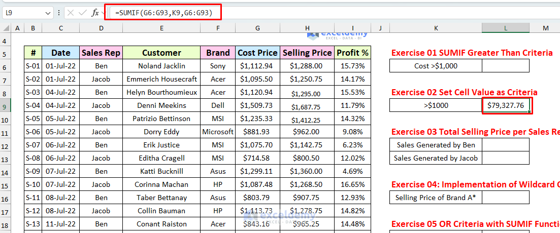
Attached the Excel File:
Practice Exercises for SUMIF.xlsm
Please verify that the values in G6:G93 are numeric and match the criteria in K9 cell exactly, without extra spaces or formatting differences.
Regards
ExcelDemy
Hello Brea Kelley,
Yes, you can auto populate venue prices in Column G of the Events sheet based on the venue listed in Column F by using the VLOOKUP function.
Use the following formula:
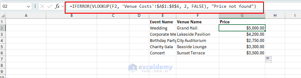
=IFERROR(VLOOKUP(F2, ‘Venue Costs’!$A$1:$B$6, 2, FALSE), “Price not found”)
Change the cell reference of of Venue Costs sheet based on your data.
Download the Excel file:
Auto Populate Value from Another Sheet.xlsx
Regards
ExcelDemy
Hello Dear,
You are most welcome. We are glad to hear that our resources are fantastic to test your Excel skills from different aspects. Keep learning Excel with ExcelDemy!
Regards
ExcelDemy
Hello Damien Connolly,
Yes, setting the variable Q to 7 in the VBA code means the loop will start from the 7th sheet, skipping sheets 1 through 6. The number 7 is used to specify where the data consolidation begins, so only sheets from the 7th onward will be included. This choice allows you to omit the first six sheets from the consolidation process. You can adjust the number if you want to include or exclude different sheets.
Regards
ExcelDemy
Hello Chad Sellers,
Thank you for your feedback! You’re absolutely right—thank you for catching that! The correct range to sum Daniel’s marks should indeed be =SUM(C5:F5), which sums the marks across all subjects for Daniel. I’ve updated the article to reflect this change, ensuring it matches the subsequent structured reference example. I appreciate your attention to detail and for bringing this to my attention!
Regards
ExcelDemy
Hello Chad Sellers,
Thank you for your feedback! You’re correct that structured table references typically apply to the same row, which can cause confusion after sorting changes the row order. I’ve updated the article to include a section that addresses how structured references behave after sorting and how to maintain consistent references to the same cell even when the row order changes.. You can use INDEX-MATCH combination or the XLOOKUP function to maintain references correctly after sorting. Your input is greatly appreciated!
Regards
ExcelDemy
Hello Joe,
Yes you can create a new cell style of your choice in Excel. In our article we have shown the steps to craete customized new cell style.
How to Create New Cell Styles in Excel
Excel provides the flexibility for users to create custom cell styles.
Steps:
For example, we can demonstrate this with a fill color such as “Gold Lighter 80%“.
After creating the style, you can easily apply it to selected cells using the Cell Styles option from the Home tab.
Custom cell styles are available only in the specific workbook where they were created.
Regards
ExcelDemy
Hello Rat,
It is possible to return a single value based on muliple values of another column. You can do it by using combination of the nested IF and OR functions without needing six separate formulas.
Use the following formula and drag the fill handle down to apply the formula to the rest of the cells in Column B.
=IF(OR(A2=”Red”, A2=”Orange”, A2=”Yellow”), “Warm”, IF(OR(A2=”Green”, A2=”Blue”, A2=”Purple”), “Cool”, “”))
The formula uses OR to check if the color in Column A matches any “Warm” colors (Red, Orange, Yellow) and returns “Warm”; if it matches any “Cool” colors (Green, Blue, Purple), it returns “Cool”. If none of these are true, it returns an empty value.
Regards
ExcelDemy
Hello Shibani Agrawal,
You can use our sample supply chain data modify it based on your requirements.
Download the Excel file:
Dataset of Supply Chain: Sample Supply Chain Dataset.xlsx
Hello Nidhi,
You are most welcome. Thanks for reading our article. Keep learning Excel with ExcelDemy!
Regards
ExcelDemy
Hello Georg,
You are most welcome. Glad to hear that you found our article great and useful. Yes, this article will help you to know everything about Scatter Chart.
Keep learning Excel with ExcelDemy!
Regards
ExcelDemy
Hello Vanessa,
You will need to extend the grouping manually to add new columns to an existing grouping without removing and reapplying the grouping. Follow the steps below to do so:
1. If your current group is collapsed, click the plus sign (+) next to the grouped columns to expand them.
2. Select the new columns that are adjacent to the existing grouped columns.
3. Go to the Data tab >> from Outline group >> select Group.
Now, Excel will automatically add the new columns to the existing group.
Regards
ExcelDemy
Hello David,
You are most welcome. Thanks for your feedback! The INDEX is an array function it recalculates every time there’s a change in the referenced data, especially if you’re working with large datasets for these reasons the file may slowdown. Though OFFSET is volatile function, but in some cases, calculates faster based on the data structure and size.
If your dataset is extensive, you might see better performance with OFFSET.
It’s great to hear that OFFEST is more efficient for your data type. Keep learning Excel with ExcelDemy!
Regards
ExcelDemy
Hello Mate,
You are most welcome. We are glad to hear that the you found the article helpful. The AutoFit shortcut method is really a time saver. Please try this method in your Excel project.
Thanks for your appreciation. Keep learning Excel with ExcelDemy!
Regards
ExcelDemy
Hello Mr. John,
You are most welcome. Thanks for your appreciation. Keep learning Excel with ExcelDemy!
Regards
ExcelDemy
Hello Amber,
It is possible to find and delete multiple values at once. To delete the first occurrences of duplicate values you can use a helper column to find out those values then apply filter to delete it.
Insert the following formula in a helper column:
=IF(COUNTIF(A2:A12, A2) > 1, IF(COUNTIF(A$2:A2, A2)=1, “Delete”, “Keep”), “Keep”)
It will check the name appears more than once. If it does, it marks the first occurrence with “Delete” and subsequent duplicates with “Keep.” For unique names it will also return “Keep”.
Now, to apply filter to your data from Data tab >> select Filter.
Then select Delete from helper column.
Finally, select all the names and press on Delete.
Download the Excel file:
Remove Duplicates First Occurences.xlsx
Regards
ExcelDemy
Hello Candy Neal,
To count how many users were active during June 2024, you can use a formula that checks if the active date is before or equal to the end of the month and if the inactive date (if it exists) is after the beginning of the month.
Insert the following formula in cell D2 and drag it down:
=IF(AND(B2<=DATE(2024,6,30), OR(C2="", C2>=DATE(2024,6,1))), 1, 0)
If you want to use it for other months change the date range in the formula.
To count total active users, insert the following formula in E2 cell:
=SUM(D2:D6)
Download the Excel file:
Count Total Active Users.xlsx
Hello Enamul Sekh,
You can download the Excel file free of cost just by providing your valid email address. All the answers are given in the Excel file. To get the files go to the Top 100 MCQ of Excel section of this post and enter your email address. Then check your email immediately after to get the download links.
Please insert your name and email address then click on Download button.
Best Regards
ExcelDemy
Hello Puri Nabaraj,
Thank you so much for your kind words! We’re glad to hear that our resources and blogs have helped you learn Excel formulas in such a short time. Your support motivates us to keep providing valuable content. Keep up the great work, and feel free to reach out if you have any questions or need further assistance!
Thanks again for your valuable feedback. Keep learning Excel with ExcelDemy!
Regards
ExcelDemy
Hello Jerry Boor,
Thank you for pointing that out! The $50,000 interest would indeed be for the entire year, not just one day’s interest. The formula and method used are correct, but the value for time was incorrectly set, which caused the confusion. I have since updated the article to reflect the correct time value (1/365) for daily interest. I appreciate your input in helping to ensure the accuracy of the content. Please feel free to check out the revised version of the article. Thanks again for your valuable feedback!
Regards
ExcelDemy
Hello Okto,
You are most welcome. Glad to hear that the formula was great to you. We always try to provide the best useful working formulas to ease your works.
Keep learning Excel with ExcelDemy!
Regards
ExcelDemy
Hello Dear,
Thanks for your appreciation! Glad to hear that the Excel templates are helpful for organizing your tax calculations. Feel free to reach out if you need any further assistance while working on your tax returns. Your feedback means a lot!
Keep learning Excel with ExcelDemy!
Regards
ExcelDemy
Hello Paul,
You are most welcome. Glad to hear that the budget sheet is helpful for you. Keep learning Excel with ExcelDemy!
Regards
ExcelDemy
Hello Maeenuddin Khan,
Glad to hear your appreciation. Thank you so much for your kind words! It’s great that the explanation helped you with finding a suitable analytical tool in Excel for your research. It’s always rewarding to know that the content makes a positive impact. If you have any further questions or need more guidance, feel free to reach out anytime. Keep up the great work with your research!
Regards
ExcelDemy
Hello Jon Peltier,
We appreciate your input. The base values in the stacked waterfall chart are calculated by starting with an initial base of 10,000 and adjusting each subsequent month’s base based on the sales flow. The base values are correctly calculated by considering the net change (positive minus negative values). The chart is intended to reflect cumulative totals, not simply stacked values. However, I appreciate your input and will ensure that this methodology is explained more clearly to avoid any confusion.
Regards
ExcelDemy
Hello,
Thanks for your feedback! While it’s true that three of the methods involve opening Excel, we included them to cater to users who may already have Excel open or prefer built-in Excel tools. The aim was to offer a variety of approaches for different user needs. However, if you’re strictly looking for methods that avoid opening Excel, the PowerShell and third-party tool methods are the best fit. We appreciate your thoughts and will keep this in mind for future articles.
Regards
ExcelDemy
Hello Antony,
You are most welcome. Glad to hear that helped you to solve your problem. If you have any more questions, feel free to ask!
Keep learning Excel with ExcelDemy!
Regards
ExcelDemy
Hello Monica,
Yes you will need to use Option 2 to show time in legend.
To handle a pie chart with time values and show those times in the legend, follow these steps given below:
1. Format you time data as time in Excel.
2. Next, use Method 2 from the article, which involves adding a helper column that combines both the time data and category labels.
3. Create your pie chart using this combined helper column as the legend, ensuring that the time is displayed as part of the legend entries.
This will allow you to show both time and categories in the legend effectively.
Regards
ExcelDemy
Hello Mohammad Afzal,
Glad to hear that you learned well. Our aim is to help you learn Excel easily. Keep learning Excel with ExcelDemy!
Regards
ExcelDemy
Hello Deanna,
Thank you! We are glad to hear your appreciation. If you don’t know the start date yet, you can set up the formula to reference the cell where the start date will be entered later. This way, once you input the start date, the calculation will automatically update. You can set up your sheet and place all the required formulas then based on your input calculation will happen automatically.
Let us know if you need further help!
Regards
ExcelDemy
Hello ExcelUser1,
Thank you for your feedback! The article primarily focuses on different methods to paste or display content, which may not fully address issues with copying merged cells directly. The challenge often lies in Excel’s limitations when copying merged cells.
If you’re facing specific issues with copying, we recommend trying unmerging cells before copying, or using VBA as outlined in the article. If this doesn’t resolve your issue, feel free to share more details, and we’ll be happy to assist further!
Regards
ExcelDemy
Hello Duncan,
The problem occurs because both the pivot table and its associated chart are copied and pasted into the email body simultaneously, overlapping each other. To resolve this, you should separate the chart from the pivot table when copying. You will need to adjust the code to specifically copy the range of cells containing the pivot table, ensuring that it does not include the chart.
We updated the VBA code where a Boolean parameter (includeChart) was added. When set to False, it will delete the chart shapes before exporting the image to ensure that only the pivot table is copied.
In the PasteRangeinMail subroutine, this parameter is set to False, so charts are excluded by default.
You can adjust the includeChart parameter as needed to ensure that only the pivot table is included in the email body.
Regards
ExcelDemy
Hello Pat Grappe,
It might be a version difference or an issue with Excel’s settings. You can try the following steps:
1. Ensure that the cells where the labels will be printed are selected.
2. Go to the Home tab in Excel.
3. Click on the Borders option in the Font group, and choose the desired border style from the dropdown.
If the Grid option is not visible, this workaround will still allow them to set borders properly.
Regards
ExcelDemy
Hello Michael,
You are most welcome. Keep learning Excel with ExcelDemy. We provided a formula to auto populate events from entry data to calendar sheet.
Regards
ExcelDemy
Hello Michael,
You are most welcome. You can auto populate events in the calendar sheet from your entry data sheet but Excel formulas has limitations over handling multiple overlapping events. Formulas will concatenate multiple events into a single cell, but each overlapping event will be separated by a line break or other delimiters.
You can use the following formula in your event cell to auto populate events.
=IFERROR(TEXTJOIN(CHAR(10), TRUE, FILTER(‘Entry Data’!$B$2:$B$100, (‘Entry Data’!$D$2:$D$100 <= B10) * ('Entry Data'!$D$2:$D$100 + 'Entry Data'!$C$2:$C$100 - 1 >= B10) * (‘Entry Data’!$E$2:$E$100 = 8) * (‘Entry Data’!$F$2:$F$100 = 2024))), “”)
Based on Month please change the Month Number and Cell reference for each month and each cell.
If an event spans multiple days, the formula will check if the current day falls within the event duration and will display the event in the cell. If multiple events occur on the same day, they will all be concatenated in the same cell.
Download the Excel file:
Monthly Event Chart
Regards
ExcelDemy
Hello Mill,
The VBA code is tailored to operate within a specific workbook context and may not be compatible as a stand-alone Excel Add-in without some adjustments. Add-ins typically work across multiple workbooks, so you need to use the modified code to ensure it can handle different active workbooks, rather than just ThisWorkbook.
To make this VBA code work as an add-in, follow the steps given below:
1. Replace references to ThisWorkbook with ActiveWorkbook.
2. Create a new module within the VBA editor and place your code there. This is necessary for turning it into an add-in.
3. Once the code is ready, save the workbook as an Excel Add-in (.xlam) file..
4. Install and test the add-in to verify that it works across different workbooks.
Now, this you can use this code as an add-in. If any further issues arise, you can refine the code further depending on their specific needs.
Regards
ExcelDemy
Hello Jennifer Almeida,
In our existing VBA code, the previously stored values in the output cell are overwritten when a new selection is made. This happens during the Button_Click event when the new selection is written directly into CheckListOutput, replacing the previous value.
To preserve previous selections, we adjusted the logic so that the newly selected value is appended to the existing content rather than overwriting it. Here’s an update to your code:
Regards
ExcelDemy
Hello Wulan Ramayani,
To develop you excel skill learn and practice the exercises given below.
Excel Data for Practice Free Download
Excel Practice Exercises PDF with Answers
Explore these categories you will find out more data entry practice here: Data Entry Practice Test & Quiz
Interview Questions with Excel Topics
MCQ Questions on MS Excel
To develop your skill from beginner to advanced level you can explore our Learn Excel page.
Regards
ExcelDemy
Hello Jason Ngo,
Thanks for your suggestion, we appreciate it deeply.Enabling Excel 4.0 macros and restarting the file should indeed help with resolving the #block error. Your step-by-step explanation is really helpful, especially the reminder to close and reopen the file for the changes to take effect. Much appreciated.
Regards
ExcelDemy
Hello Babajide,
Thanks! We are glad to hear that you found it great. We try our best to provide excellent services. Keep learning Excel with ExcelDemy!
Regards
ExcelDemy
Hello Yufeng,
You are most welcome. Thanks for your appreciation it means a lot to us. Keep learning Excel with ExcelDemy!
Regards
ExcelDemy
Hello Dennis,
Thank you for the feedback! To use dynamic dropdowns, using UserInterfaceOnly = True can indeed allow macros to run while keeping the sheet protected. The UserInterfaceOnly setting allows VBA to make changes, but it doesn’t allow certain actions like adding or modifying data validation directly on a protected sheet.
Here’s an updated VBA code that temporarily unprotects the sheet to apply the data validation and then reprotects it:
Regards
ExcelDemy
Hello Heather,
May be the problem is related to Excel’s limitations when applying multiple conditional formatting rules or when handling a large range with VBA. This could be causing the code to slow down or enter an infinite loop. A possible solution is to break the range into smaller sections or optimize the code by limiting the number of FormatConditions applied at once.
Here, I’m Reviewing the loop logic and error handling, could also help prevent the program from freezing.
I used FormatConditions.AddUniqueValues with xlDuplicate to highlight duplicates directly.
Then used the Chunk size logic is retained to process large ranges in smaller sections.
All the ranges are based on our existing Excel sheet.
Use the updated VBA code:
Regards
ExcelDemy
Hello Kay D,
The issue with using 248 rows in your INDEX and SMALL formula is not the problem, as Excel can handle thousands of rows in such functions. It sounds like the issue may be related to how the INDEX and SMALL functions are handling the range of cells. If the formula is getting values from the wrong row, there could be a mismatch between the row numbers used in the SMALL function and the actual row numbers in your data.
Make sure that the ranges in your formula are correctly aligned with your dataset. Double-check that the criteria and ranges match, and ensure there are no offset errors.
Adjust the “-4” ensure that the offset corresponds to the starting row of your range. Try modifying the offset if necessary, depending on your data structure.
Check Criteria Range: Ensure the $C$5:$C$12 range is aligned with your criteria column.
You can share your formula if you want. We can help to troubleshoot it further!
Regards
ExcelDemy
Hello Stephen,
It’s not possible to set the color or grayscale options to appear as default when opening the print menu in Excel. Those settings are controlled at the system level via your printer preferences. In Excel, you can still access these settings, but each time you print, you’ll need to manually adjust the color options unless they’ve been preset in your system’s printer properties.
To adjust your printer preferences at the system level rather follow these steps:
1. Go to your Devices and Printers settings in your operating system.
2. Right-click on your printer >> select Printing Preferences, and configure your preferred settings there.
This will set your defaults across all programs, including Excel, without needing to change them each time in the print menu.
Regards
ExcelDemy
Hello Miran,
You are most welcome. To split data into separate sheets based on different columns like Sales Person or Region, you will need to adjust the VBA code.
Here is the updated VBA code:
In the first InputBox insert the dataset range.
Then choose the column number to spilt the data.
Regards
ExcelDemy
Hello Demba,
We have created a dataset for Customs Compliance Monthly Report in Excel based on your given fields.
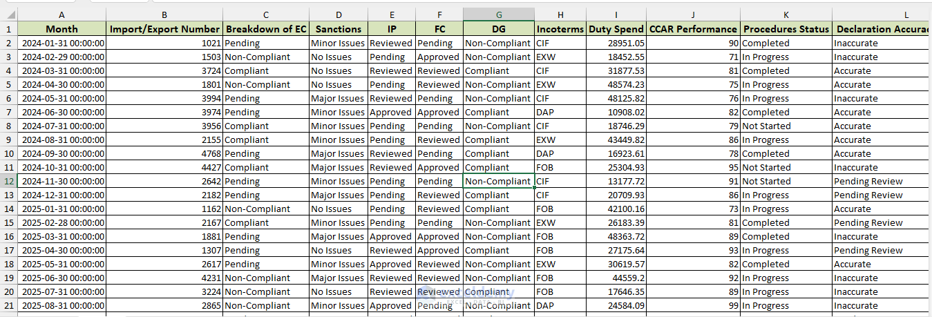
Download the Excel file from here : Customs Compliance Monthly Report.xlsx
Regards
ExcelDemy
Hello Joost,
Hope you are doing well. Thank you for your feedback! Applying the same color to all bars in a group might not be ideal if they represent different years or categories. It’s better to use different colors or shades for clarity. This helps in distinguishing the data within the group more effectively. That’s why we avoided same color across the grouped bar chart.
But if it is helpful to you to visualize the bars then you can do it.
As Excel doesn’t automatically apply the same color across the grouped bar chart categories. You can manually adjust the colors by selecting each data series and applying the same color.
Follow the steps to do so:
1. Click on one of the bars you want to change.
2. Right-click and select Format Data Series.
3. Choose Fill and pick your desired color.
Repeat for each data series to maintain consistent coloring across all groups.
Regards
ExcelDemy
Hello Fritz,
The VBA code is working fine in our end.
Make sure to follow all the steps:
Create the drop down list first then place the VBA code in that sheet.
Double-check that the VBA code is correctly placed in the Sheet where the data validation with drop down list exists.
Also, ensure that there are no conflicts with other existing macros or data validation settings. If the issue persists, try testing the code in a new worksheet to see if it works there.
You can download our workbook for testing purpose: Selecting Multiple Options from Drop Down.xlsm
Regards
ExcelDemy
Hello Kevin,
Great to hear that it worked great. You’re absolutely correct Method 6 returns the row numbers where there’s a match, not the number of rows. We updated the article to correct this typo. Appreciate your attention to detail!
Thanks for your feedback. Keep exploring Excel with ExcelDemy.
Regards
ExcelDemy
Hello Balaji,
All the solutions are available in the Solution sheet of the Excel Workbook. Excel file is given in the Download practice Workbook section.
All the solutions are given part by part in the Solution sheet.
Regards
ExcelDemy
Hello Craig,
Yes. It is possible to download the graph. We always provide a ready to use Excel file in our Download section.
Please download the chart from here: Plot Sieve Analysis Graph.xlsx
Regards
ExcelDemy
Hello Mel,
You can use a custom formula in Excel’s conditional formatting to highlight cells in column B and C based on the presence or absence of specific text (deed) in another column G.
Follow the steps given below:
1. Select the range in columns B and C that you want to format.
2. Go to Home > Conditional Formatting > New Rule.
3. Choose “Use a formula to determine which cells to format”.
4. Enter the following formula: =ISERROR(SEARCH(“deed”,$G1))
This will highlight cells in columns B and C if the corresponding cell in column G does not contain “deed.”
5. Set the formatting style and click OK.
Regards
ExcelDemy
Hello Femi,
Thanks for your appreciation. You will need to update the report card based on the student ID then you will be able to print the results for all names of the list.
While changing the name please update marks of each student.
Regards
ExcelDemy
Hello Don,
There is no formula in cell C5, and cells C5 only contain marks. So, there’s no risk of creating a circular reference. The steps should work as described. Can you please check out this is the right article you commented?
Thanks for your feedback.
Regards
ExcelDemy
Hello Saad,
Thanks for your feedback. Apologies for the typo. You are right the correct answer should be “Alexander – Home Theater”. We’ve updated it now. Thanks for your understanding!
Regards
ExcelDemy
Hello Mohammad Afzal,
It’s great decision. ExcelDemy can help you to start your learning. Our website contents are designed to help you learn Excel from basics to advanced.
Follow our Learn Excel page here you will find all the topics related to Excel.
Explore all the Tutorial categories to explore more. We also provide courses to learn Excel technology.
Regards
ExcelDemy
Hello Iliyana,
Hope you are doing well. Sorry to hear your problem. While executing the code you need to follow the steps.
First, open the sheet from where you want to copy the filtered values. Suppose you selected Dataset sheet.
Go to Developer tab >> from Macros >> select Sub Copy_AutoFiltered_VisibleRows_NewSheet().
Now, you will get the filtered values in Sheet3. Make sure you have created a sheet named Sheet3 otherwise you will get the error out of “Subscript out of range” and it will show a yellow fill in Worksheets(“Sheet3”).Range(“a1”).PasteSpecial Paste:=xlPasteAll line.
If you want to get your filtered values in your desired sheet. Just name it in the code.
If you still find the issue please attach a image or error name and it’s description. We will be happy to help you.
Regards
ExcelDemy
Hello Nithin,
Your deep learning projects some of the tasks you can accomplish in Excel, such as organizing data and performing calculations. But the full scope of your project would require additional software and programming.
1. You will need to use Optical Character Recognition(OCR) software to scan the question paper and answer sheet.
It will recognize and extract question numbers and their corresponding marks.
2. Then use Python scripts to process OCR output, map questions to answers, and recognize marks.
3. Finally you can use Python libraries like pandas and openpyxl to create and format an Excel file with the extracted data.
Regards
ExcelDemy
Hello Lorcan,
As all the steps are sequential the issue of not seeing the option to add dynamic content in the ‘To’ box when creating the ‘Send an Email (v2)’ action in Power Automate might be due to a bug or a temporary glitch.
Try the following steps to troubleshoot,
1. Refresh your browser or reopen Power Automate.
2. Clear your browser cache.
3. Ensure all fields are properly configured before the ‘Send an Email (v2)’ action.
4. Check for any updates to Power Automate.
If the issue persists, consider reaching out to Microsoft support for further assistance. You can try our 2nd method until the issue is solved.
Regards
ExcelDemy
Hello Alex,
You are most welcome. Thanks for your appreciation, it’s great to hear that you found the article helpful.
To get cell color from a specific cell you can use the user defined function.
Copy paste the VBA code:
Use this function in a cell to reference the specific cell from another sheet whose color you want to retrieve.
You also can follow this article: How to Get Cell Color in Excel
Regards
ExcelDemy
Hello Don,
It seems you’re facing issues with dynamic named ranges on Mac OS Excel v16.16. Our article is written based on based on Windows OS Excel 365.
Here are some steps you may try to troubleshoot the problem.
Date =OFFSET(Combined!$A$2, 0, 0, COUNTA(Combined!$A:$A)-1, 1)
Value =OFFSET(Combined!$B$2, 0, 0, COUNTA(Combined!$B:$B)-1, 1)
When replacing the series formula in your chart, ensure it looks like this.
=SERIES(“Combined”, Combined!Date, Combined!Value, 1)
If automatic updates are causing errors, manually update the data ranges:
1. Right-click on the chart and select Select Data.
2. Edit the series and input the named ranges manually.
Ensure that your Excel on Mac OS is up to date. Sometimes, these issues are resolved with software updates. There might be compatibility issues between Windows Excel 365 and Mac OS Excel v16.16. Dynamic named ranges sometimes behave differently across platforms.
Regards
ExcelDemy
Hello Kurt Kruger,
Our existing code generate Code 128 barcodes, primarily focusing on Code 128B, and can switch to Code 128C for efficient numeric encoding when needed. Modified the existing VBA code to include Code 128A encoding, which includes upper-case letters, control characters, and special characters. The start, checksum, and stop characters are added to generate a valid Code 128A barcode.
Regards
ExcelDemy
Hello Imtiaz,
You’re welcome! I understand that working with VBA may seems complex if you’re not familiar with it. Here’s a step-by-step guide to use the VBA code:
To open the VBA editor press Alt + F11.
In the VBA editor, go to Insert >> select Module. This will create a new module where you can paste the VBA code.
Copy and Paste the First Code in the module.
Next, in the VBA editor, find Sheet1 (or the name of your sheet where you’ll enter the date) in the Project Explorer on the left side.
You can also Double-click on Sheet1 to open its code window.
Now, copy paste the 2nd code in the Sheet.
Make sure to replace “$A$1” with the actual cell reference where you will be entering the date if it’s different.
Now, go back to your Excel sheet. Enter a date in the specified cell (e.g., A1) on Sheet1 and check if the date gets updated in the corresponding cell on all other sheets.
Regards
ExcelDemy
Hello Jim Green,
You are most welcome. Your appreciation means a lot to us. We are grateful that you found the insights helpful. Keep learning Excel with ExcelDemy!
Regards
ExcelDemy
Hello David Silberberg,
To apply the conditional formatting in column H based on the data of column F and it’s formatting you need to follow the steps given below:
To highlight the entire column H.
Go to the Home tab >> click Conditional Formatting >> select New Rule.
Choose Use a formula to determine which cells to format.
Enter the formula =ISNUMBER(SEARCH(“BofA”, $F2)).
To Set Formatting:
Click on Format.
Set the font and fill colors to match those used in column F for “BofA”.
Then, select OK to apply the formatting.
Again, click OK to apply the rule.
By following this step, any cell in column H will automatically reflect the same font and fill colors as column F when the corresponding cell in column F contains “BofA”.
Download the Excel file:
Copy Conditional Formatting.xlsx
Regards
ExcelDemy
Hello Falak Niaz,
Certainly! Your formula correctly extracts the data between the two dashes. Your feedback and suggestion will be helpful for other users.
If you want you can simplify it by using MID function.
=MID(B29, FIND(“-“, B29) + 1, FIND(“-“, B29, FIND(“-“, B29) + 1) – FIND(“-“, B29) – 1)
Thanks for sharing your formula.
Regards
ExcelDemy
Hello Yngwie,
Before proceeding to advance level to develop your Excel skills you can explore the given links. Download the files from the articles to learn and practice the exercises.
Excel Data for Practice Free Download
Excel Practice Exercises PDF with Answers
Explore these categories you will find out more data entry practice here: Data Entry Practice Test & Quiz
Interview Questions with Excel Topics
MCQ Questions on MS Excel
To develop your skill from beginner to advanced level you can explore our Learn Excel page.
Regards
ExcelDemy
Hello Errol,
Great to hear that you found the video interesting. You will need to use VBA code and several steps to create a form in Excel for a library database that updates with data from worksheets, step by step procedures:
Create the worksheets (Books and Users). Design the form with text boxes and buttons. Then run the VBA code.
Step 1: Organize Data in Worksheets
Books Worksheet: Include columns such as Book ID, Title, Author, Genre, etc.
Users Worksheet: Include columns such as User ID, Name, Class, etc.
Step 2: Create the Form
Insert Form Controls.
Use Insert > Form Controls to add text boxes and buttons for input.
Step 3: Add VBA Code to Handle Data
Open the VBA Editor (Alt + F11).
Insert a New Module and copy paste the following code.
Importing Books
Importing Users
Adding New Book
Adding New User
This setup will allow you to efficiently manage your library database, importing data from worksheets and updating forms without manual entry for each record.
Regards
ExcelDemy
Hello Jennifer,
Thank you for your feedback. Our template auto-calculates the “DATE DUE” field based on your inputs, ensuring accuracy and efficiency. All input fields are editable, and no password is required.
We just freeze the row-20 two maintain the template dashboard.
To unfreeze it select row-20 >> from View >> select Unfreeze Panes.
Please check our how to use this template section carefully.
If you encounter specific issues, please share the details, including screenshots, so we can assist you better. We are committed to resolving any problems you may face.
Regards
ExcelDemy
Hello Adnan,
You are most welcome. We are glad to hear that you found this article extremely helpful. Keep learning Excel with ExcelDemy!
Regards
ExcelDemy
Hello Matador,
You are most welcome. We are glad to hear that you found the lesson easy and helpful! Thank you for your kind words. If you have any more questions or need further assistance, feel free to ask! Keep learning Excel with ExcelDemy!
Regards
ExcelDemy
Hello Bjangaiah,
Thanks for your appreciation. We are glad to hear that it was helpful to you. We always try our best to provide a proper and detail explanation. Keep learning Excel with ExcelDemy!
Regards
ExcelDemy
Hello Kenneth,
To auto sort the list alphabetize based on their names you can use the SORT function.
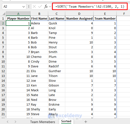
Here, I used the SORT function to sort your data automatically each time you enter new player name.
=SORT(‘Team Memebers’!A2:E100, 2, 1)
To make a team used the TEXTJOIN and FILTER function.
=TEXTJOIN(“, “, TRUE, FILTER($A$2:$A$21, $E$2:$E$21=H1))
If you are comfortable with VBA then you also can use the code instead of SORT function.
Insert the code in the Team Members sheet.
Download the Excel File:
Auto Sort Team Members Name and Assign Team
Regards
ExcelDemy
Hello Joe Bardswich,
Your statement is not clear whether you referring to AutoFill or Auto Calculations. I am providing solution for both of them.
If AutoFill is not working please check out this article: Excel Autofill is Not Working
If Auto Calculations is not working check out this article: Excel Formulas Not Calculating Automatically
If this solutions doesn’t work for you, please provide more details about what you were able to do before and what is not working now. You can attach dummy image of your dataset. This will help me give you the most accurate advice.
Regards
ExcelDemy
Hello Djeeni,
Thank you for your feedback. We appreciate it. Expanding the VBA example to handle ranges with multiple columns is a fantastic suggestion. Here’s a detailed approach:
To handle multiple columns, iterate through each row within the specified range and concatenate cell values (e.g., combining first name and last name) to form a unique string for each row. Use this concatenated string as a key in a scripting dictionary to ensure each value is stored only once, maintaining uniqueness.
After processing all rows, output the unique values from the dictionary to the specified location in the worksheet.
This approach will efficiently identify and store unique combinations of cell values across multiple columns. We will update the article with the detailed VBA code example to illustrate this process. Thank you for your valuable input.
Regards
ExcelDemy
Hello Rechelyn Cañete,
You are most welcome. To develop your Excel skills you can explore the given links. Download the files from the articles to learn and practice the exercises.
Excel Data for Practice Free Download
Excel Practice Exercises PDF with Answers
Explore these categories you will find out more data entry practice here: Data Entry Practice Test & Quiz
Interview Questions with Excel Topics
MCQ Questions on MS Excel
To develop your skill from beginner to advanced level you can explore our Learn Excel page.
Regards
ExcelDemy
Hello Johnrey Cambaya,
You are most welcome. To develop your Excel skills you can explore the given links. Download the files from the articles to learn and practice the exercises.
Excel Data for Practice Free Download
Excel Practice Exercises PDF with Answers
Explore these categories you will find out more data entry practice here: Data Entry Practice Test & Quiz
Interview Questions with Excel Topics
MCQ Questions on MS Excel
To develop your skill from beginner to advanced level you can explore our Learn Excel page.
Regards
ExcelDemy
Hello Marissa Coetzee,
Sorry to hear your problem. This issue may caused due to regional settings or data formatting differences. Make sure your regional settings in Excel match those of your teammate.
Also, check for any leading/trailing spaces or non-numeric characters in your data. Cleaning your data using the Text to Columns or Find & Replace features might help.
Or you can use the VALUE function to convert the values in number then use the Get Data option.
Clean your data then use proper data format before using the Get Data option.
Regards
ExcelDemy
Hello David McKenna,
To adjust the column width you need select right icon. As there appears multiple icons based on position when you select a whole column. Perhaps you selected the copy icon instead of width icon.
To adjust width you must place the cursor in the column header then select the plus icon with arrow. Please check the image to see the icon.
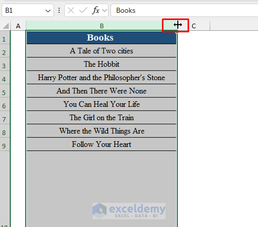
To copy the column you need to select the icon marked in the given image.
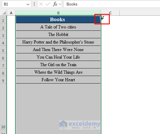
Regards
ExcelDemy
Hello Enrique Arizmendi,
You are most welcome. Your appreciation means a lot to us. We are glad to hear that our article helped you to explore the possibilities of Excel. Keep learning Excel with ExcelDemy!
Regards
ExcelDemy
Hello Ebsa,
You are most welcome. To create a forest plot for categories and sub categories follow the steps given below.
Create your dataset with the following columns.
Category: The main category.
Subcategory: The subcategories under each main category.
Estimate: The effect estimate or mean value for each subcategory.
Lower CI: The lower bound of the confidence interval for each estimate.
Upper CI: The upper bound of the confidence interval for each estimate.
First, insert a Scatter Plot:
1. Select the columns for the subcategories and the estimates.
2. Go to Insert > Chart > Scatter > Scatter with Straight Lines and Markers.
Next, add Error Bars:
1. Click on the chart to activate the Chart Tools.
2. Go to Chart Tools > Layout > Error Bars > More Error Bar Options.
3. Select Both for direction and specify Custom for the error amount.
4. Use your Lower CI and Upper CI values for the custom error amount. Enter these values manually.
Next, Customize the Chart:
1. Add titles, labels, and adjust the axes as needed.
2. To add a vertical line at the point of no effect (usually zero or one), draw a line using the Shapes tool and place it at the appropriate point on the X-axis.
Next, Format the Chart:
1. Adjust the colors, line styles, and marker shapes to differentiate between categories and subcategories.
2. Add data labels if necessary for clarity.
Finally, Group Categories and Subcategories:
1. If you have multiple main categories, use different colors or shapes to represent each main category.
2. Add a legend to help differentiate between the categories.
By following these steps, you can create a clear and informative forest plot in Excel that displays categories with their respective subcategories, including confidence intervals for each estimate.
Regards
ExcelDemy
Hello Kristal,
Thanks for sharing this solution! It’s a great solution for highlighting overdue dates and those due within 30 days.
To avoid formatting blank cells, you need to use a more specific condition.
You can apply conditional formatting with the formula: =AND(A1<>“”, A1
This formula will check if the cell is not blank (A1<>“”), and then it will verify if the date is less than 30 days from today (A1. This ensures that only non-blank cells with dates within the next 30 days are formatted.
If you need further assistance please let us know. Keep learning Excel with ExcelDemy.
Regards
ExcelDemy
Hello Rich Courtney,
The green circle with an arrow at the tip of your pointer is related to the Caps Lock feature. This is a new feature in Safari on macOS to indicate that Caps Lock is enabled.
To turn off or disable this feature, you can try the following steps:
System Preferences:
1. Open System Preferences.
2. Go to Keyboard.
3. Under the Keyboard tab, look for any settings related to Caps Lock or Keyboard shortcuts and disable any relevant options.
Safari Preferences:
1. Open Safari.
2. Go to Safari > Preferences (or press Cmd + ,).
3. Look for any settings that might be related to this feature under the Advanced or Accessibility tabs and disable them if found.
Accessibility Settings:
1. Open System Preferences.
2. Go to Accessibility.
3. Look for any settings related to keyboard or pointer and disable any features related to Caps Lock notifications.
Sometimes reinstalling the application can help resolve unexpected behavior.
If none of these steps work, consider reaching out to Apple Support for more detailed assistance. They might provide a specific way to disable this new feature or offer an alternative solution.
Regards
ExcelDemy
Hello Alvin,
This VBA macro sends an email if the date in a selected range matches Today’s date. It prompts the user to select a range of cells and checks each cell in the range. If a cell’s value matches the current date, it asks the user for the email subject, sender, recipient, CC, BCC, and message body. It then uses Outlook to send the email with the provided details.
In your date range you must include the date which will match Today’s date.
To understand the logic I added a debugging option here:
If you need further customization or have a specific dataset, please provide more details about how you want the VBA code to work.
Regards
ExcelDemy
Hello Rav,
You are most welcome. To add the headers along with the searched values use the following updated VBA code:
Output:
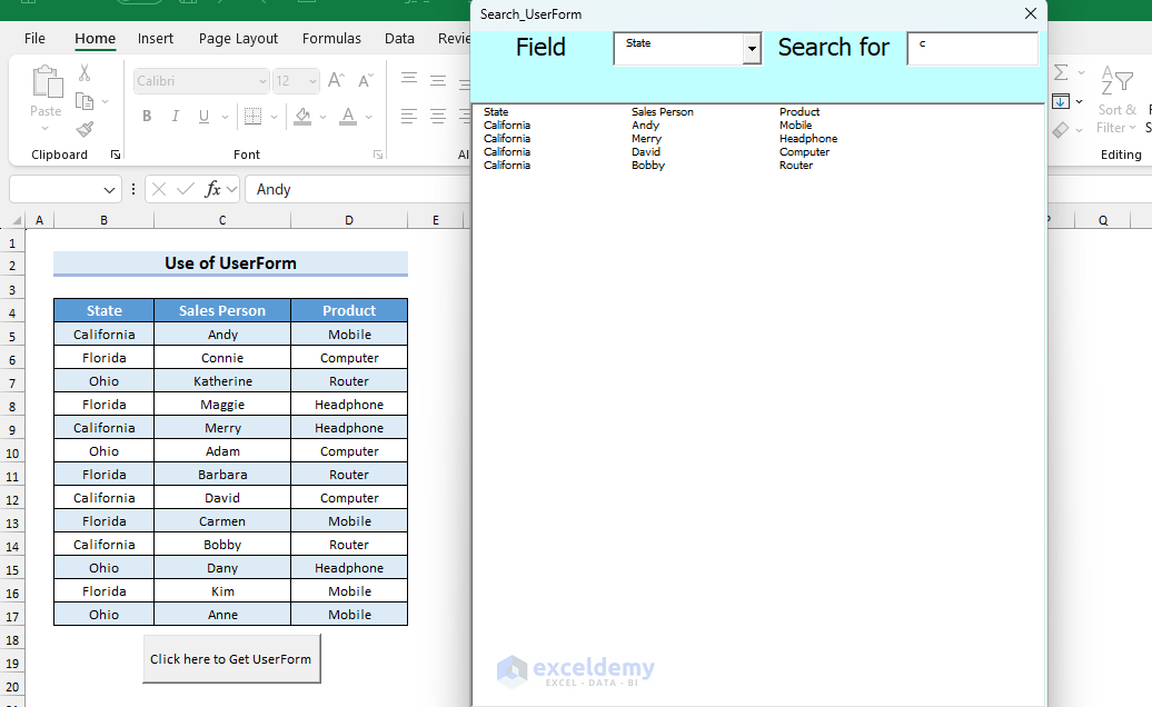
Regards
ExcelDemy
Hello Undent,
Sorry to hear your problem. But our Method-1 is working perfectly. Can you check your IF condition based on your case or dataset.
Here, I’m attaching a image where IF function returns the values based on the conditions.
If you want you can share your case here.
Regards
ExcelDemy
Hello Gordan,
It’s a common issue with Excel pivot tables and slicers. You can follow the steps given below to maintain the formatting of your pivot table when using slicers:
Use Cell Styles:
Instead of relying on pivot table styles, try applying cell styles to the pivot table.
Select the cells you want to format, go to the “Home” tab, and choose “Cell Styles“. This approach can help preserve formatting when slicers are used.
Use a VBA Code:
If you’re comfortable with VBA, you can use a VBA script to reapply formatting whenever the pivot table is updated.
Right-click the sheet tab with your pivot table, choose “View Code,” and paste this code into the worksheet module.
Create a Custom Pivot Table Style:
You can create a custom pivot table style that includes all your desired formatting. To do this:
Click on your pivot table.
Go to “Design” > “PivotTable Styles” > “New PivotTable Style.”
Define your style, including fonts, colors, borders, etc.
Apply this custom style to your pivot table.
By trying these methods, you should be able to maintain your pivot table’s formatting even when using slicers. Let me know if you need more specific guidance on any of these topic.
Regards
ExcelDemy
Hello Veekay,
You are most welcome. We try to summarize all possible solutions so that you can use any of the solution based on your dataset type. Keep solving Excel problems with ExcelDemy.
Regards
ExcelDemy
Hello Morgan Trevino,
Checked method-2 to confirm the issue. Method-2 is working perfectly:
To ensure that only overdue dates are highlighted using method 2, please check the conditional formatting formula used. The formula should compare the dates with today’s date.
You also can use the formula: = A1 (replace A1 with the appropriate cell reference for your dates). This formula will highlight only the dates that are earlier than today’s date.
If you need further guidance, please share the exact formula you used so I can help you correct it.
Regards
ExcelDemy
Hello Larry,
Based on your previous comment.
To add the date to column K of the matched row of TCN of column B, you will need to use the Date function. It will provide the current date.
Here, I updated the VBA code to add the date. Make sure to place this code in the appropriate worksheet module where you are scanning the barcodes.
Regards
ExcelDemy
Hello Guy,
You cannot open the same Excel sheet in safe mode without closing it first. Safe mode is designed to start Excel without add-ins or other customizations, which requires restarting the application. If you are experiencing issues with a specific sheet, try saving your work, close Excel, then reopen it in safe mode using the Ctrl key method:
1. Press and hold the Ctrl key.
2. While holding Ctrl, click on the Excel icon to open it.
3. A prompt will appear asking if you want to start Excel in safe mode. Click Yes.
This method allows you to open a new instance of Excel in safe mode while keeping your current sheet open.
Regards
ExcelDemy
Hello Larry,
To add the date to column K of the matched row of TCN of column B, you will need to use the Date function. It will provide the current date.
Here, I updated the VBA code to add the date. Make sure to place this code in the appropriate worksheet module where you are scanning the barcodes.
Regards
ExcelDemy
Hello Srivatsan Guru,
You are most welcome. It’s great to hear that it was helpful to you. Keep learning Excel with ExcelDemy.
Regards
ExcelDemy
Hello AMG,
You are most welcome. It’s great to hear that Method-7 was helpful to you and it worked perfectly. Keep learning Excel with ExcelDemy.
Regards
ExcelDemy
Hello Jerry,
Method-3 is working perfectly. To get the page number in a proper way you need to insert the page number first. Follow the given steps to insert the page number in a selected cell.
First select a cell >> go to Developer tab >> from Macros >> select Page_Number_Selected_Cell().
It will insert the page number.
Remember to select the cell sequentially to add page numbers.
Output:
Regards
ExcelDemy
Hello Michel Claes,
You are most welcome. Thank you for your feedback! I’m glad you found the article helpful.
Static oldval(6 To 10) As Variant: Declares a static array oldval to store previous values of cells F6 to F10, so the values persist between subroutine calls.
The variable “oldval” is initialized at the first run of the subroutine to store the initial cell value before any changes occur. It’s updated only when a change is not detected to retain the previous value for comparison. This way, it can accurately identify when a change happens in the cell value.
If you have any further questions or need more clarification, feel free to ask!
Regards
ExcelDemy
Hello Rolands,
You are most welcome. Thank you for your feedback! I’m glad the solution worked for you. Replacing Target.Address with Target.Column = 5 is a great adjustment for your setup with multiple drop-down cells in column E. It’s wonderful to hear that it continues to work even for newly created and copy-pasted rows.
We used Target.Address initially to target specific cells, making it easy to apply the method to designated areas. This approach provides precision and control, especially useful for varying drop-down list configurations.
Regards
ExcelDemy
Hello Melody,
Thank you for your interest! Unfortunately, we are unable to provide a PDF version of the content from the Learn Excel page on ExcelDemy. But you can always access and study the material directly on our website at any time. If you have any specific topics or questions, feel free to let us know, and we’ll be happy to help!
Regards
ExcelDemy
Hello Hari Lalam,
You are most welcome. It is great to hear that the Google Sheets method accomplished your task. Keep learning Excel with ExcelDemy.
Regards
ExcelDemy
Hello Johnson Helen,
You are most welcome. We are glad to hear that it was really helpful to you. In our Practice Test & Quiz category you will find out more data entry practice here: Data Entry Practice Test & Quiz
Keep learning Excel with ExcelDemy.
Regards
ExcelDemy
Hello Raif,
You are most welcome. We are glad to hear that our example worked for you. You can explore more article related to VBA. Keep learning Excel with ExcelDemy.
Regards
ExcelDemy
Hello Samwel Gurt,
You are most welcome. We are glad to hear that our article is excellent and satisfying to you. You can explore more article related to these topic. Keep learning Excel with ExcelDemy.
Regards
ExcelDemy
Hello Samwel Gurt,
Thank you so much. We are glad to hear that you loved our article. You can explore more article related to these topic. Keep learning Excel with ExcelDemy.
Regards
ExcelDemy
Hello Me,
You are most welcome. Your appreciation means a lot to us. You can explore more article related to these topic. Keep learning Excel with ExcelDemy.
Regards
ExcelDemy
Hello Tony Jin,
You are most welcome. Your appreciation means a lot to us. You can explore more article related to these topic. Keep learning Excel with ExcelDemy.
Regards
ExcelDemy
Hello Matthew Richard Raison,
The problem with the VBA code not working for a different roster template could be due to differences in the sheet structure. While using different sheet structure update the VBA code according to you new sheet:
1. Ensure the cells for month and year are correctly referenced (W2 and AC2).
2. Adjust the CopyToSheet subroutine to match the layout and structure of your specific roster sheet.
3. Verify that the new sheet created is an exact replica by manually inspecting the VBA code to ensure all ranges and cell references align with your roster’s layout.
Make these adjustments, and the code should work as intended.
Regards
ExcelDemy
Hello Claudia Sgiarovello,
On our end the VBA code is working perfectly. Rechecked the code to confirm it.
Make sure you replace the curly quotation marks with straight quotation marks to avoid syntax errors in VBA. If the problem persists, double-check the name of the range “CheckListOutput” to ensure it matches exactly with what is in your Excel workbook.
1. Ensure all quotes are straight quotes (“).
2. Check that “CheckListOutput” matches the actual named range in your Excel workbook.
3. Verify that “checkList” matches the name of your ActiveX listbox control.
If these steps don’t resolve the issue, consider providing more details about any specific error messages or behaviors you’re encountering.
Regards
ExcelDemy
Hello Muskan Gadodia,
To Load/Export the table into an Excel worksheet follow these steps:
Select the sheet name (Departmental Sheet) and Right-Click on the sheet. Then, select Load To.
Import Data dialog box will pop up
From there select Table.
Then select the location where you want to put the data. Here, selected A1 cell.
Finally, data is exported to a table.
You will get the steps in our updated article also.
Regards
ExcelDemy
Hello Anonymous,
Thank you for your feedback! I’ve updated the document to include detailed explanations for each example, showing exactly how each formula works step-by-step. This should make it easier for you to understand how to adapt the formulas for your own spreadsheets.
I’m glad the initial examples were helpful, and I hope the added explanations will provide the deeper understanding you’re looking for. If you have any more questions or need further clarification, please feel free to ask. Happy spreadsheeting!
Regards
ExcelDemy
Hello Idrissa A.Kamara,
You’re most welcome! I’m glad to hear that the materials and tutorial have been helpful in enhancing your Excel skills and intelligence. Your dedication to learning and improvement is truly inspiring. God bless you as well, and if you ever need further assistance or have more questions, feel free to reach out. Keep up the great work!
Keep leaning Excel with ExcelDemy.
Regards
ExcelDemy
Hello Bob,
Thank you for bringing this to our attention. Our template is designed to handle various loan amounts and interest rates. I’ve checked the template again by changing loan amount, interest , tenure etc and it’s working perfectly. I will request you to check, How to Use This Template part of the article.
Templates’ intial image:
Different Loan Amount and Interest Rate:
Another changes:
It sounds like there might be a formatting or input error causing the #VALUE! error. Please ensure that:
Loan Amount and Interest Rate Formats: The values are entered as plain numbers without any special characters or spaces. For example, enter 200000 for $100,000 and 8 for an interest rate of 8%.
Correct Cells: The values are being entered in the correct cells specified for loan amount and interest rate.
If you’ve checked these and are still encountering issues, please feel free to share a screenshot or more details about the error. We’ll be happy to assist further.
Thank you for your patience and understanding.
Regards
ExcelDemy
Hello Faye,
The formula provided calculates the straight-line (great-circle) distance between two points, not accounting for roads, highways, or specific travel routes. This is why you notice a discrepancy when comparing it to Google Maps or Bing, which calculate driving or walking distances along actual travel paths.
The straight-line distance is the shortest path over the earth’s surface, which does not reflect the true travel distance that might involve various roads and pathways.
Thanks for commenting and asking questions! It’s great that you’re diving into the details and eager to learn. No worries, it’s not a dumb question at all! Learning these differences is part of the process. Keep up the good work!
Regards
ExcelDemy
Hello Andrew,
There is a way to set up to be used repeatedly and routinely but for that you will need to install Adobe Acrobat SDK this is necessary for controlling Acrobat via VBA. Then you will need to use VBA code and Task Schedular.
Copy the VBA code to find the PDF file from a directory.
Now, set up the Task Scheduler:
1. Open Task Scheduler
Search for “Task Scheduler” in the Windows Start menu and open it.
2. Create a Basic Task
o Click on “Create Basic Task…” in the Actions pane.
o Name your task (e.g., “Automate PDF to Excel”) and provide a description.
o Click “Next”.
3. Set Trigger
o Choose when you want the task to start (e.g., Daily, Weekly).
o Click “Next” and set the start date and time.
o Click “Next”.
4. Set Action
o Choose “Start a program” and click “Next”.
o In the “Program/script” field, enter the path to the Excel executable (e.g., C:\Program Files\Microsoft Office\root\Office365\EXCEL.EXE).
o In the “Add arguments (optional)” field, enter the path to your Excel workbook (e.g., “C:\path\to\your\workbook.xlsm”).
o Click “Next”.
5. Finish
o Review your settings and click “Finish”.
6. Configure Task
o Locate your new task in the Task Scheduler Library.
o Right-click it and select “Properties”.
o Go to the “Actions” tab and click “Edit”.
o In the “Add arguments (optional)” field, add the following to run the specific macro:
/e /mImportPDFData
o Click “OK” and then “OK” again to save your changes.
This setup will automatically open the Excel file and run the specified macro at the scheduled times.
Regards
ExcelDemy
Hello Sid,
You can use the Application.OnKey method to assign a macro to a specific key. To handle the “Insert” key, you need to use the correct key code.To use the Insert key as an event along with Application.OnKey do the followings:
Copy paste the following code in the Moduel:
Then copy paste the following code in ThisWorkbook:
The Workbook_Open event, will set the Application.OnKey to assign the “Insert” key to this macro and the Workbook_BeforeClose event, clear the key assignment when closing the workbook.
Regards
ExcelDemy
Hello Paolo,
You are most welcome. We are glad to hear that you found our solution easy and efficient. Keep finding Excel solutions with ExcelDemy.
Regards
ExcelDemy
Hello Nate,
You are most welcome. We are glad that our solution worked perfectly for you. Keep finding Excel solutions with ExcelDemy.
Regards
ExcelDemy
Hello Bhabani,
Please fill out this form properly to get the FREE Advanced Excel Exercises with Solutions
I received the exercise sheet via email after filling out the form.
Regards
ExcelDemy
Hello Karin Williams,
You are most welcome. Thanks for your appreciation, it means a lot to us. We are glad to hear that you found our article most comprehensive. Keep learning Excel with ExcelDemy.
Regards
ExcelDemy
Hello Keith Miller,
I understand your frustration with transitioning from MSQuery to Power Query, especially after being familiar with MSQuery for so long. The learning curve can be a bit daunting, but the good news is that Power Query is incredibly powerful and can handle the task you described quite efficiently.
To join two tables into one data set without resorting to Access or using numerous VLOOKUP formulas, Power Query is indeed your best bet.
Please follow this article to Combine Two Tables Using Power Query in Excel
To create relationship between two tables you can follow the given steps too:
Let’s say, we have two tables describing different products ordered by some customers from separate addresses and their respective prices.
I have created the first column named Customer Information with headings: Customer ID, Name, and Address.
Another table named Order Information has headings like: Name, Product, and Price.
It is noticeable that there must be a common column to create a relationship between the tables.
Here, I will show the method of creating relationships using Pivot Table. In order to demonstrate this method, proceed with the following steps.
Steps:
I have named the first table Customer and the second table Order.
So, these are the steps you can follow to create a relationship between tables using the Pivot Table option.
Read More: How to Create Data Model Relationships in Excel
Download the Excel File: Creating Relationship Between Tables.xlsx
Regards
ExcelDemy
Hello SH,
The VBA code is working perfectly. Similarities of two columns are highlighted in Red color.
Here, I am uploading a video of VBA code:
Video of VBA code Highlighting Similarities
Kindly use the following code again:
Please click on Yes to highlight the similarities.
Regards
ExcelDemy
Hello Daz C,
Making AllTaskList sheet a table is not an issue. May be Named Range is not working properly that’s why VLOOKUP is not getting the lookup values.
Please, check the tasklist from Named Manager.
Go to Formulas >> from Defined Names >> select Name Manager.
Check the Tasklist contains =’AllTaskList (2)’!$B:$G
N.B: You can change your list based on your sheet.
Here, I made the AllTaskList a table to check either it’s a problem or not.
Then, checked the Task Detail sheet to see VLLOKKUP is working or not.
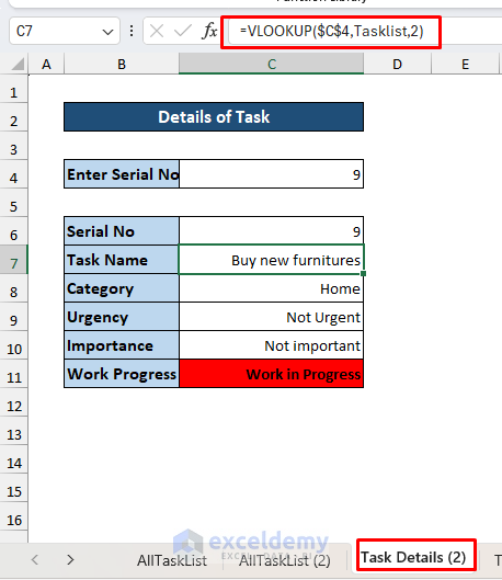
Here VLOOKUP is working perfectly.
I am uploading the updated Excel file, please download it from here:
Creating a Task Tracker Using Table.xlsx
Reagards
ExcelDemy
Hello Leo Mulhern,
The Excel file is working fine in my end. I updated the stocks name and it is working.
Track Stock Prices:
Updated Stock Prices:
Again, I uploaded the Excel file for you:
Track Stocks in Excel (Updated).xlsx
If new file keeps shutting down, try these steps to fix the issue:
Update Excel: Make sure Excel is up to date.
Disable Add-Ins: Open Excel in Safe Mode (hold Ctrl while opening Excel), then disable add-ins from File -> Options -> Add-Ins.
Repair Office: Go to Control Panel -> Programs -> Programs and Features, find Microsoft Office, right-click, select Change, and choose Quick Repair.
Regards
ExcelDemy
Hello Flipmode,
Thank you for your feedback and for highlighting the importance of accurate formulas. However, the provided formula in the article is giving correct results for the USD to EUR conversion as shown in the example table. The VLOOKUP formula used is correctly referencing the exchange rate and multiplying it with the USD value. Here, we are converting currencies from USD to any other currency.
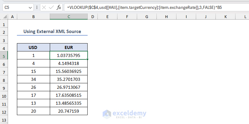
USD to EURO:
USD to ARS:
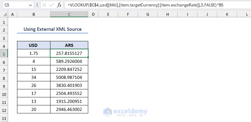
N.B: In our article we used exchange rate data of 9/27/2022
Thank you for your feedback. If your specific examples work for reversing the lookup, then it’s a wonderful solution. We appreciate your suggestions and hope other users find your insights useful. Thanks for your contribution!
Regards
ExcelDemy
Hello Julie Binks,
Based on your table you can match data to return sales. Use the following formula to get data based on partial name.
=VLOOKUP(“*”&E5&”*”,B4:C11,2,FALSE)
Here is the sample data with output:
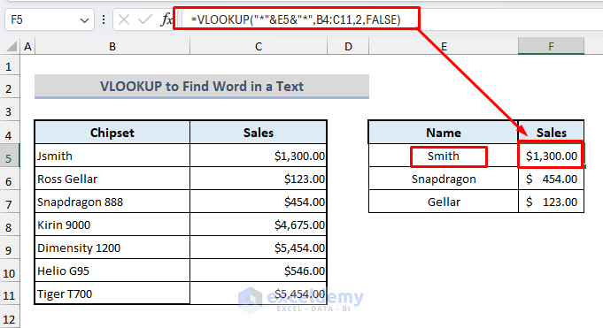
Regards
ExcelDemy
Hello Ahmed,
You are most welcome. Thanks for your appreciation it means a lot to us. Keep learning Excel with us.
Regards
ExcelDemy
Hello JM Kim,
Here, created a single bar chart horizontal with two values Active an Inactive or 1 and 0 which is displayed with different color and x axis it time value.
Download the Excel File: Single Horizontal Bar Chart Showing Active Inactive Status.xlsx
Regards
ExcelDemy
Hello Kumar Chavan,
You need to create two sheets to present your expenses.
Firstly, create Income and Expenditure Account sheet to record all incomes and expenditures for the year, including the deferred income adjustment for repairs.
Then, create Balance Sheet to present the assets, liabilities, and equity as of the year-end date.
Here is your Example Format: Template for Income and Expenditure Account and Balance Sheet.xlsx
Regards
ExcelDemy
Hello JZ,
NYSE ticker SNOW for Snowflake is included in Excel database.
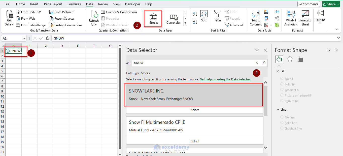
To get the data follow the steps below.
Insert SNOW in any cell then click on Stocks from Data tab.
You will get all the data by selecting the fields.
Regards
ExcelDemy
Hello Imtiaz,
To do so you need to use two VBA code in your Excel workbook. One in the Module to update date and another in the first sheet where you will update the date. Make sure to replace “Sheet1” with the actual name of the sheet where you will enter the date, and “A1” with the cell reference where the date is located.
Copy and paste the following VBA code into the new module:
To automatically update the date whenever the date is changed, you need to use the Worksheet_Change event.
In the VBA Editor, double-click the sheet where you will enter the date (e.g., Sheet1) in the Project Explorer window.
Then, paste the following code:
Again, replace “$A$1” with the actual cell reference where the date is located.
Now, whenever you change the date in the specified cell on your primary sheet (e.g., Sheet1), the date will automatically be updated in the corresponding cell on all other sheets.
VBA code will assume that the date is located in the same cell on each sheet.
Regards
ExcelDemy
Hello Ramesh Satyanarayanamurthy,
To search multiple text in single cell by using the IF,ISNUMBER and SEARCH function, use the following formula:
=IF(ISNUMBER(SEARCH(“Service”, B5)), “Server Status”, IF(ISNUMBER(SEARCH(“Application”, B5)), “Application Status”, IF(ISNUMBER(SEARCH(“Connect”, B5)), “Connectivity”, IF(ISNUMBER(SEARCH(“CPU Utilization”, B5)), “CPU Utilization”, “”))))
Output:
Regards
ExcelDemy
Hello Jacob,
Thanks a lot for sharing this solution. Defining the validation string using a ListObject is indeed a smart approach. By turning the data into a table, we can avoid manually editing column addresses and ensure the code remains functional even if the table moves.
I appreciate the suggestion to make both sets of data into tables for easier referencing. This will definitely help in maintaining the code’s robustness and flexibility.
Regards
ExcelDemy
Hello Patrick Raimond,
To use the iterative formula you need to do the following changes in Excel options
Enable Iterative Calculations:
First, go to File > Options > Formulas.
Then, select Enable iterative calculation.
Today’s Output:
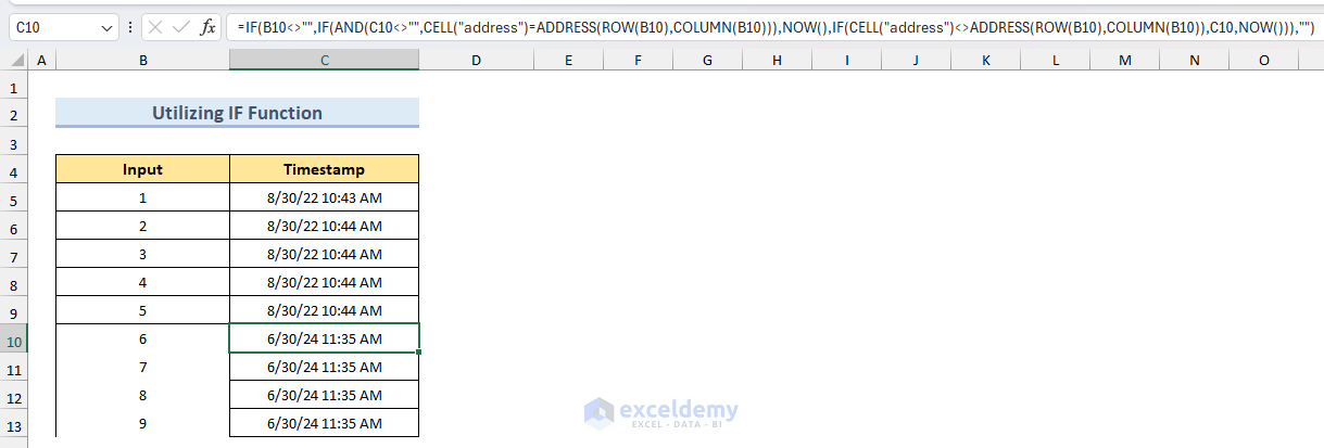
Regards
ExcelDemy
Hello Tejas,
If the search cell has multiple criteria, you can use the following formula:
=TEXTJOIN(“, “, TRUE, IF(ISNUMBER(SEARCH($E$4:$E$5, B4)), $E$4:$E$5, “”))
It checks if any of the values in the criteria range are found within the text in cell B4. The SEARCH function identifies the presence of these values, and ISNUMBER confirms their existence. The IF function returns the matching values, while TEXTJOIN concatenates them into a single string, separated by commas, ignoring empty results. This allows multiple matches to be displayed in one cell.
Regards
ExcelDemy
Hello D.A.
Here updated the VLOOKUPCMT function and named VLOOKUPCMT_New where handled threaded comments in newer versions of Excel.
Added deletion of existing threaded comments and handling of threaded comments
To ensure that the function can handle both old-style comments and new threaded comments. Use the following updated code:
This will copy the comments. To copy notes use the previous code.
Regards
ExcelDemy
Hello Neet,
You are most welcome. We are glad to hear that our article solved your problem. Thanks for your appreciation. Keep learning Excel with us.
Regards
ExcelDemy
Hello Tara Man,
You are most welcome. We are glad to hear that you got what you needed. Keep learning Excel with us.
Regards
ExcelDemy
Hello Muhammad Farg,
Yes, there are multiple ways to merge data under same headlines. In this article we showed how to merge sheets step by step: How to Merge Sheets in Excel
You can follow this VBA code to merge the data and arrange it at the same time under one headline:
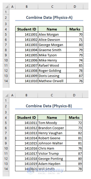
Before using the code make sure both of your sheets contains the same headings.
Sheet1 & Sheet2:
Output:
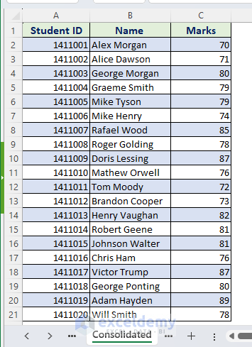
Excel File: Merge Data in Same Headings.xlsx
Regards
ExcelDemy
Hello Agung,
To handle the leave request for next month we updated our existing template. Added a new sheet to enter leave requests. Based on this sheet modified the existing formulas to consider leave request.
You will get a roaster template without leave request:
=IF(AND(INDEX(LeaveRequests!$B$2:$B$11,MATCH(‘Roster 24”7’!$B$8,LeaveRequests!$A$2:$A$11,0),1)<=E$7,INDEX(LeaveRequests!$C$2:$C$11,MATCH('Roster 24''7'!$B$8,LeaveRequests!$A$2:$A$11,0),1)>=E$7), IF(OR($C8=””,E$7=””), “”,IF(D8= “”,C8, INDEX(Settings_Shift_Legend,IF(MATCH(RIGHT(D8,2),Settings_Shift_Legend,0)+1>COUNTA(Settings_Shift_Legend),1,MATCH(RIGHT(D8,2),Settings_Shift_Legend,0)+1))))&”- On leave”, IF(OR($C8=””,E$7=””), “”,IF(D8= “”,C8, INDEX(Settings_Shift_Legend,IF(MATCH(RIGHT(D8,2),Settings_Shift_Legend,0)+1>COUNTA(Settings_Shift_Legend),1,MATCH(RIGHT(D8,2),Settings_Shift_Legend,0)+1)))))
Here is the formula to show leave requests:
=IF(AND(INDEX(LeaveRequests!$B$2:$B$11,MATCH(‘Roster 24”7’!$B$8,LeaveRequests!$A$2:$A$11,0),1)<=E$7,INDEX(LeaveRequests!$C$2:$C$11,MATCH('Roster 24''7'!$B$8,LeaveRequests!$A$2:$A$11,0),1)>=E$7), IF(OR($C8=””,E$7=””), “”,IF(D8= “”,C8, INDEX(Settings_Shift_Legend,IF(MATCH(RIGHT(D8,2),Settings_Shift_Legend,0)+1>COUNTA(Settings_Shift_Legend),1,MATCH(RIGHT(D8,2),Settings_Shift_Legend,0)+1))))&” – Leave Req”, IF(OR($C8=””,E$7=””), “”,IF(D8= “”,C8, INDEX(Settings_Shift_Legend,IF(MATCH(RIGHT(D8,2),Settings_Shift_Legend,0)+1>COUNTA(Settings_Shift_Legend),1,MATCH(RIGHT(D8,2),Settings_Shift_Legend,0)+1)))))
Download the Excel File: 24×7 Shift Roaster Template with Leave Requests
Regards
ExcelDemy
Hello Guadalupe Valdez,
To get value from another workbook you can use the VLOOKUP function.
In Worksheet2:
In cell B2 Enter the following formula:
=IFERROR(VLOOKUP($A2,[Worksheet1.xlsx]Sheet1!$A$2:$D$5, 2, FALSE), “”)
This formula looks up the Slot number in A2 of Worksheet2 in the range A2
of Worksheet1. The IFERROR function will return an empty string if no match is found.
Then, drag the formula down to A440 cell.
Use the same formula by changing the column number for First and Last name.
In cell C2 of Worksheet2, enter the following formula:
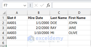
=IFERROR(VLOOKUP($A2, [Worksheet1.xlsx]Sheet1!$A$2:$D$440, 3, FALSE), “”)
In cell D2 of Worksheet2, enter the following formula:
=IFERROR(VLOOKUP($A2, [Worksheet1.xlsx]Sheet1!$A$2:$D$440, 4, FALSE), “”)
Final Output:
Here, I am attaching the Excel Files:
Worksheet1.xlsxhttps://www.exceldemy.com/wp-content/uploads/2024/06/Worksheet2.xlsx
Worksheet2.xlsx
Regards
ExcelDemy
Hello Michelle,
Yes, you can add a check in the VBA script to see if the search box is empty before proceeding with the search. If the search box is empty, the subroutine can exit early without performing any operations, preventing the script from unnecessarily processing all the data and causing lag.
Here, added IsEmpty() and a simple comparison to an empty string (“”) to check if the Search_Cell is empty before running the rest of the code.
If the search cell is empty, it displays a message box alerting the user and exits the subroutine early with Exit Sub.
Regards
ExcelDemy
Hello Derek,
We are glad to hear that our solution helped you. Thanks for your appreciation. Keep learning Excel with us.
Regards
ExcelDemy
Hello Yulissa Alvarez,
Based on your given scenario created a dummy dataset to auto populate one sheet values based on information from another sheet.
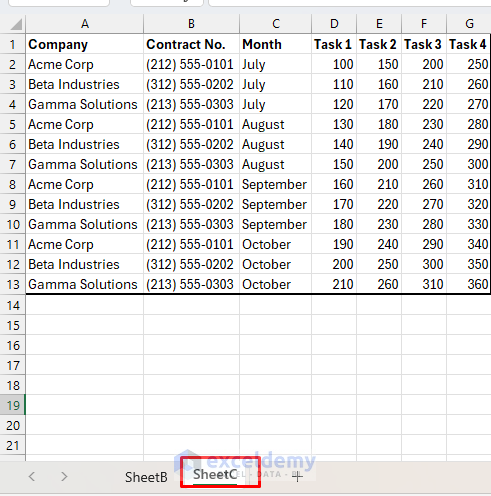
Here I used INDEX-MATCH functions to get data from another sheet dynamically.
Use the following formulas:
Task1: =INDEX(SheetC!$D$2:$D$13, MATCH(1, (SheetC!$A$2:$A$13=SheetB!$B2) * (SheetC!$B$2:$B$13=SheetB!$C2) * (SheetC!$C$2:$C$13=SheetB!$D2), 0))
Task2: =INDEX(SheetC!$E$2:$E$13, MATCH(1, (SheetC!$A$2:$A$13=SheetB!$B2) * (SheetC!$B$2:$B$13=SheetB!$C2) * (SheetC!$C$2:$C$13=SheetB!$D2), 0))
Task3: =INDEX(SheetC!$F$2:$F$13, MATCH(1, (SheetC!$A$2:$A$13=SheetB!$B2) * (SheetC!$B$2:$B$13=SheetB!$C2) * (SheetC!$C$2:$C$13=SheetB!$D2), 0))
Task4: =INDEX(SheetC!$G$2:$G$13, MATCH(1, (SheetC!$A$2:$A$13=SheetB!$B2) * (SheetC!$B$2:$B$13=SheetB!$C2) * (SheetC!$C$2:$C$13=SheetB!$D2), 0))
If you want to add more task just change the cell-refernce.
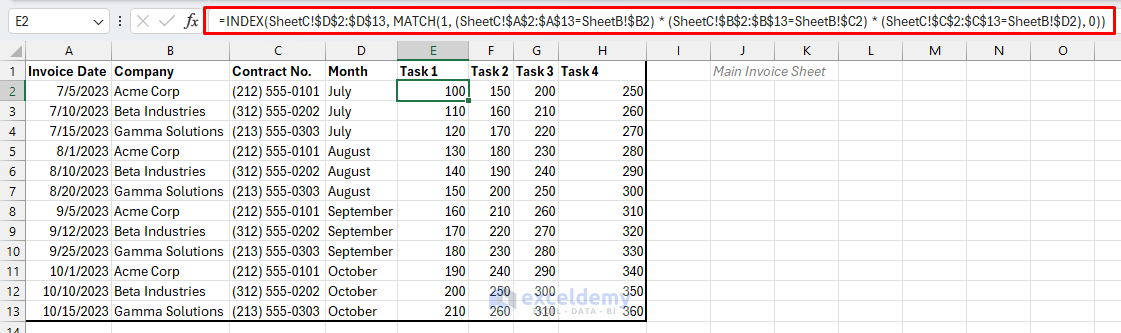
Output:
You can Download the Excel file:
Auto Populate Values from Another Sheet
Regards
ExcelDemy
Hello Michelle,
The “Run-time error ‘9’: Subscript out of range” occurs when a specified sheet or range does not exist. Please check the sheet names and ranges in your Searched_Sheets and Searched_Ranges arrays are correctly spelled and match exactly with your Excel workbook.
I made some changes in the code to check whether sheets and ranges exist in your Excel workbook.
Make sure to update this according to your Excel workbook:
Searched_Sheets = Array(“Dataset 1”, “Dataset 2”) # Update it with your sheet name.
Searched_Ranges = Array(“B5:F23”, “B5:F23”) # Update it with your ranges.
Added SheetExists function it will check if a sheet exists before accessing it.
Error Handling will check for the existence of sheets to prevent “Subscript out of range” errors.
Regards
ExcelDemy
Hello Daniele,
Buongiorno! Se la colonna della data è formattata correttamente ma la tabella pivot mostra ancora le date ogni giorno senza raggrupparle per mesi o anni, prova questi passaggi:
Assicurati che tutte le date siano nel formato corretto e che non siano presenti valori di testo.
Fai clic con il pulsante destro del mouse su qualsiasi data nella tabella pivot, seleziona “Gruppo” e scegli il raggruppamento desiderato (ad esempio, mesi o anni).
Se il problema persiste, controlla le opzioni avanzate in Excel per assicurarti che l’opzione “Raggruppa date nel menu Filtro automatico” sia abilitata.
Segui questi articoli per risolvere il tuo problema:
[Fix] Cannot Group Dates in Pivot Table
Excel Pivot Table Not Grouping Dates by Month (4 Solutions)
How to Group Dates in Pivot Table: 7 Methods
Good morning! If your date column is correctly formatted but the pivot table still shows dates daily without grouping by months or years, try these steps:
1. Ensure all dates are in the correct format and there are no text values.
2. Right-click any date in the pivot table, select “Group,” and choose the desired grouping (e.g., months or years).
If this doesn’t work, check the advanced options in Excel to ensure ‘Group dates in the AutoFilter menu’ is enabled.
If you still face problem, check out this articles:
[Fix] Cannot Group Dates in Pivot Table
Excel Pivot Table Not Grouping Dates by Month (4 Solutions)
How to Group Dates in Pivot Table: 7 Methods
Regards
ExcelDemy
Hello Lucy Jackson,
Thanks for your appreciation, it means a lot to us. We are glad to hear that our article solved your problem. Keep learning Excel with us.
Regards
ExcelDemy
Hello Tracy,
Thanks for your appreciation, it means a lot to us. Keep learning Excel with us.
Regards
ExcelDemy
Hello Zayaan,
You are most welcome. Thanks for your appreciation. We have a category of pivot table and data analysis. We will create more pivot table for data analysis and power pivot. Keep learning Excel with us.
Please explore our this section.
Pivot Table in Excel
Data Analysis in Excel
Power Pivot
Regards
ExcelDemy
Hello Bryan,
You are most welcome. Thanks for your appreciation. Keep learning Excel with us.
Regards
ExcelDemy
Hello Praveen
As we used digit limit in our existing code that’s why it is showing this warning.
Don’t worry! We have updated the existing VBA user-defined function to overcome the problem and work with much larger numbers. In the Indian numbering system, we use terms such as Thousand, Lakh, Crore, Arab, Kharab, Neel, Padma, and Shankh to express large numbers. So, the user-defined function will return the word-converted result using these terms. Moreover, we will use an Excel built-in TEXT function to get accurate results for huge numbers.
Use the following updated code:
=AdvancedWord(TEXT(A1,"#.00"))Hopefully, you have found the solution you were looking for. I have attached the solution workbook as well. Good luck.
DOWNLOAD SOLUTION WORKBOOK
Regards
ExcelDemy
Dear,
Thanks for your appreciation. Keep learning Excel with us.
Regards
ExcelDemy
Hello Lisa,
We are glad to hear that our article helped you. It means a lot to us. Keep Learning Excel with us.
Regards
ExcelDemy
Hello Alphonse
Thanks for sharing an important aspect of variable declaration. You are absolutely correct.
In VBA, when we declare multiple variables in a single line, like Dim Str1, Str2, Str3, Str4, Str5 As String, only the last variable (in this case, Str5) is declared as the specified type (String). The others (Str1, Str2, Str3, and Str4) are implicitly declared as Variant types. So, If we expect all variables to hold string values, declaring them explicitly as String ensures they behave consistently.
Why This Matters: Variants consume more memory than specific types like String. Explicit type declarations help prevent errors related to type mismatches. Moreover, string operations like concatenation might behave differently if the variable is not explicitly declared as a String. Again, If we perform validations or transformations assuming the data type is String, having a Variant could lead to bugs or incorrect results.
So, our Improved Excel VBA Sub-procedure can be following:
Thanks again for sharing your expertise in ExcelDemy Community. Stay blessed.
Regards
ExcelDemy
Hello Lisa,
Yes, you can streamline data copied from a bank statement in a Word document to an Excel spreadsheet.
Follow the steps given below:
1. Copy the data from your Word document.
2. Open Excel and paste the data into a spreadsheet.
3. Use the “Text to Columns” feature in Excel to split the data into columns based on delimiters like spaces or tabs.
4. Organize the data by month using Excel’s sorting and filtering tools.
You can follow this articles too: How to Copy from Word to Excel into Multiple Cells (3 Ways)
How to Convert Word Table to Excel Spreadsheet: 6 Quick Methods
How to Convert Word to Excel Keeping the Formatting – 2 Easy Methods
How to Convert Word to Excel with Columns (2 Methods)
Regards
ExcelDemy
Hello John Facey,
Yes, Excel has a limitation in handling very large numbers due to its floating-point arithmetic, which can lead to precision errors. When squaring 111,111,111, the correct result is 12,345,678,987,654,321, but Excel is displaying 12,345,678,987,654,300 due to this limitation. This discrepancy is because Excel can only precisely handle integers up to 15 digits. To get the exact result, consider using specialized software or programming languages that support arbitrary-precision arithmetic.
Regards
ExcelDemy
Hello Sia,
To modify the VBA code to round up the sum result to the nearest integer, you can use the Application.WorksheetFunction.Ceiling function. Use the following updated code to get your desired result:
The formula will be : =SumByColor(A1, A1:C1)
Regards
ExcelDemy
Hello Alphonse,
You are most welcome Your appreciation means a lot to us.
Regards
ExcelDemy
Hello J,
Thanks for your comment and for noticing the fact! You are right about losing conditional formatting when the pivot table is refreshed.
When a pivot table is refreshed, custom formatting will reset because the data structure may change; for example, new rows or columns might be added. Excel may not reapply the formatting rules applied to specific cells if the layout of the pivot table changes. So, in this case, you need to manually reapply the conditional formatting rules each time the pivot table is refreshed.
Regards
ExcelDemy
Hello Enrique Rafhael
Thanks for visiting our blog and sharing your problem. The existing formula returns an array containing both latitude and longitude. If you are not using Microsoft 365, you need to press Ctrl+Shift+Enter instead of pressing Enter.
However, If you want to avoid returning an array and want to get latitude and longitude individually, follow these steps:
Hopefully, following this procedure, you can avoid returning an array. Good luck.
Regards
ExcelDemy
Hello Onkar,
Please try this updated VBA code. Replace “C:\YourFolderPath\” with the path to your files. This updated code will ensures headers are copied only from the first file.
Regards
ExcelDemy
Hello Cosmin,
To fix your issue, use the following formula.
Improved Excel Formula: =INT(B5/300) & ” days ” & INT(MOD(B5/300, 1) * 5) & ” hours ” & MOD(B5, 60) & ” minutes”
Regards
ExcelDemy
Hello Rebecca,
Thanks for your compliments! Your appreciation means a lot to us.
You can create a countdown from a specific date, excluding weekends and holidays, using a combination of the TODAY, ABS and NETWORKDAYS.INTL functions in Excel.
Excel Formula: =ABS(NETWORKDAYS.INTL($C5,TODAY(),1,$C$11:$D$12))
Hopefully, you have found the solution you were looking for. You can download the workbook used to solve your problem from the following link:
CountDown Excel File.xlsx
Regards
ExcelDemy
Hello Mp3 juice,
You are most welcome. Thanks for your appreciation. Our free templates are ready to use.
Regards
ExcelDemy
Hello Valarmathi,
You are most welcome. Thanks for your appreciation.
Regards
ExcelDemy
Hello Emrah,
You are most welcome. To adapt DeepL you may use third party Add-ins, Power Query and VBA code. But VBA code will be more complex as you need to use JSON converter.
You can use the Add-ins “Text Translator for Excel”

Using Power Query with DeepL API
Use the Power Query to call the DeepL API directly from Excel.
Follow the steps given below:
Step 1: Get Your API Key from DeepL
Sign up on the DeepL website and get your API key.
Step 2: Open Excel and Launch Power Query
Open Data tab > from Other Sources > select Web.
Step 3: Configure the API Request
In the Web dialog box, enter the DeepL API URL with your query parameters,
Insert YOUR_API_KEY with your actual API key and modify the text and target_lang parameters as needed.
Then click OK.
Step 4: Transform the Data
Power Query will open a new window with the API response.
Use the available transformation tools to parse the JSON response and extract the translated text.
Finally, Close & Load to import the data back into Excel.
Regards
ExcelDemy
Hello Umeeksha Sharma,
Thank you for sharing your solution! Creating a new Excel file and importing the problematic file is indeed a practical approach. This method can help ensure the dates are correctly categorized in years and months format. If you need further assistance or have any other tips to share, feel free to let us know!
Regards
ExcelDemy
Hello IDn,
Thanks for your appreciation. It means a lot to us.
Regards
ExcelDemy
Hello Amara,
Here I’m attaching a sample dataset for CRM and Supply chain. You can modify this dataset based on your requirements.
Dataset of CRM:CRM Dataset.xlsx
Dataset of Supply Chain: Supply Chain Dataset.xlsx
Regards
ExcelDemy
Hello Abdul,
Excel file is given in the download section of the article. You also can download the template with formula from this link : Ageing Formula 30 60 90 Days.xlsx
Regards
ExcelDemy
Hello Michael George Eichbaum,
Can you please specify which portion of the article seems complex or hard to you? We will update this part for you.
But this is the easiest way to insert horizontal slicer in Excel.
Regards
ExcelDemy
Hello Nhung,
Your appreciation means a lot to us. We are glad that our article helped you to fix your issues.
Regards
ExcelDemy
Hello John,
You are most welcome. Glad to hear that it saved you from fiddling tasks.
Regards
ExcelDemy
Hello Slides Downloader,
We are glad to hear that it worked for you and you got relief from frustrating tasks. Thanks for your appreciation. It means a lot to us.
Regards
ExcelDemy
Hello Merry Gizaw,
You are most welcome.
Regards
ExcelDemy
Hello Laura,
Sorry to hear your issue. Here, I am suggesting some troubleshooting steps to resolve the problem. But I will encourage you to submit your Excel file in our ExcelDemy Forum so that we can inspect it thoroughly.
1. Remove Non-Printable Characters:
Use =CLEAN(C2) to clean the data.
2. Check for Merged Cells:
Ensure there are no merged cells in your dataset.
Data Consistency:
3. Make sure all data in Column C are of the same type (text).
4. Sort by Multiple Columns:
Use Data > Sort,
and add levels to sort by Column C first and then Column E.
5. Manual Inspection:
Check the middle section where the sort restarts for any anomalies.
6. New Worksheet:
Copy and paste the data into a new worksheet and try sorting again.
Regards
ExcelDemy
Hello Selva,
You are most welcome.
Regards
ExcelDemy
Hello Kitonski,
Here, I made some fixes. Please try this updated code:
Used the shell.Run command which is synchronous (True as the last parameter), ensuring the Python script completes before the VBA code proceeds.
Using the Now function to calculate the start and end times accurately.
To be safe used the Shell execution uses the correct quotation marks to avoid syntax errors.
Regards
ExcelDemy
Hello Hassan Ibrahim Mohammed,
Hope you are doing well. I will suggest you to go through the article again. You can download the dataset to try the calculations.
1: Likert Scale Range and Its Effect on Final Results
Here, each Likert scale response (ranging from 1 to 5) is assigned a numerical value. These values are added up for each respondent to get a total score. For example, if a respondent’s answers to five questions are 4, 3, 5, 2, and 1, the total score is 15. This summed score helps in analyzing the overall sentiment or opinion of the respondents. Higher scores indicate more positive responses, while lower scores indicate more negative responses.
2: Adding Non-Parametric Tests to Excel
To add non-parametric tests like the Mann-Whitney U test or the Kruskal-Wallis test to your Excel sheet, you can use the dataset from the article. But Excel does not have built-in non-parametric test functions, you need to manually calculate them using formulas and the Data Analysis ToolPak (If not available in Ribbon, get it from Excel options). For example, you can rank your Likert scale data using the RANK function and then apply the necessary formulas to perform the tests. It may require detailed setup and understanding of the test procedures, but it can be done effectively in Excel.
Regards
ExcelDemy
Hello Patricia,
To solve this issue:
First, add columns for monthly interest and new balance.
Then, for each debt, include columns for monthly interest and new balance.
Use the following formula to calculate monthly interest:
Monthly Interest = Previous Balance * (Annual Interest Rate / 12)
Example:
Debt 1 (D2): =C2*0.17/12
Debt 2 (H2): =G2*0.19/12
Debt 3 (L2): =K2*0.20/12
Use the following formula to calculate new balance:
New Balance = Previous Balance + Monthly Interest – Payment
Example:
Debt 1 (E2): =C2+D2-B2
Debt 2 (I2): =G2+H2-F2
Debt 3 (M2): =K2+L2-J2
Regards
ExcelDemy
Hello Sandy,
You can use this formula:
=OR(WEEKDAY([@DATE], 2) = 6, WEEKDAY([@DATE], 2) = 7)
This checks if the [@DATE] column value is a Saturday (6) or Sunday (7).
Regards
ExcelDemy
Hello Poppy Lukhele,
Could you be more specific? If possible share any sample data.
Regards
ExcelDemy
Hello Mary Grace,
Please use this updated code to get your desired result:
Here I added an input box to select the column with the names of the recipients (XRcptsName ). Then, updated the email body to include the recipient’s actual name and removed the word “text.”
Regards
ExcelDemy
Hello Paul Tupper,
Yes, we can use this formula too. Thanks for your suggestions, we really appreciate it.
Regards
ExcelDemy
Hello Paul Tupper,
Of course, you can use this formula too. Both are doing the same calculations. Our formula is simpler nothing else. Thanks for your suggestions, we really appreciate it.
Regards
ExcelDemy
Hello George Jululian,
You are most welcome.
Regards
ExcelDemy
Hello Hen,
Thanks for your appreciation.
Regards
ExcelDemy
Dear,
You are most welcome.
Regards
ExcelDemy
Hello Jeromy Adofo,
You are most welcome. please stay connected with us.
Regards
ExcelDemy
Hello Myron,
You are most welcome.
Regards
ExcelDemy
Hello Aleksandar,
You can concatenate the cell values into a single string to get one QR code from different cell values.
You can use the following code:
Regards
ExcelDemy
Hello Muhammad Afzaal Jutt,
You need to use a combination of functions like SUBSTITUTE, TEXTJOIN, FILTERXML, and SUM. Currently, Excel does not directly provide a simple formula for this without VBA.
You can use the following formula:
=SUM(FILTERXML("<t><s>" & SUBSTITUTE(SUBSTITUTE(A1, " ", "</s><s>"), "$", "") & "</s></t>", "//s[number(.)=.]"))Regards
ExcelDemy
Hello Ckwong,
To get the result as State Name. You need to use the state name column as an array of INDEX function. Just replace the cell range from C5:C12 to B5:B12.
You can use the following formula:
=INDEX(B5:B12, MATCH(TRUE, INDEX(C5:C12>700000, 0), 0))
Regards
ExcelDemy
Hello Esraa Yaseen,
You are most welcome. We are glad to help you.
Regards
ExcelDemy
Hello Prabhakar Srinivasagam,
You are most welcome. Your kind words means a lot to us. We are always here to help you.
Regards
ExcelDemy
Hello Abinsh,
You are most welcome.
Regards
ExcelDemy
Hello Jen,
Thanks for coming back, hopefully it will work this time. If it doesn’t work, you can let us know your problem in the comment section below.
Regards
ExcelDemy
Hello Usama Jamil,
You are most welcome.
Regards
ExcelDemy
Hello Atif Hassan,
Thanks for your appreciation. You can use the following formula to use XLOOKUP with tolerance level:
=XLOOKUP(TRUE, IF(ABS($C$2:$C$4 – $A$2) <= $B$2, TRUE, FALSE), $D$2:$D$4, "Not Found")
https://www.exceldemy.com/wp-content/uploads/2024/05/XLOOKUP-Based-on-Customized-Criteria.gif
Please download the Excel file for better understanding:
XLOOKUP with Tolerance Level.xlsx
Regards
ExcelDemy
Hello Danielle Davies,
You are most welcome. Your appreciation means a lot to us.
Regards
ExcelDemy
Hello Vito,
Don’t be sorry Vito. Let us know your feedback, hopefully it will work.
Regards
ExcelDemy
Hello Jose,
You are most welcome. Your appreciation means a lot to us.
Regards
ExcelDemy
Hell MM,
You are most welcome.
Regards
ExcelDemy
Hello Michael,
You are most welcome.
Regards
ExcelDemy
Hello T Althoff,
Our updated article indeed includes three templates of different cases, each addressing different scenarios. You can modify these templates to recalculate interest and principal based on irregular payment dates, they offer versatile solutions for various other scenarios.
Regards
ExcelDemy
Hello Reza Fadlilah,
Here are some articles from where you can download dataset of different types to practice your skills.
Excel Sample Data (Free Download 13 Sample Datasets)
Excel Data for Analysis (Free Download 11 Suitable Datasets)
Excel Data for Practice Free Download
Regards
ExcelDemy
Dear Ayebusiwa Oyesanmi Emmanuel,
Answers are given in the Solution sheet of Excel File which is in Download Practice Workbook section.
Regards
ExcelDemy
Hello Emon,
You can download the Cheat Sheet free of cost just by providing your valid email address. To get the files go to the “Download Excel Formulas Cheat Sheet PDF & Excel Files” section of this post and enter your email address. Then check your email to get the download links.
Best Regards
ExcelDemy
Hello Abdul,
It’s glad to hear and you are most welcome.
Regards
ExcelDemy
Hello Rhonda Rodriguez,
Thanks for your appreciation. You are most welcome.
Regards
ExcelDemy
Hello Michailmqo,
You can mail to [email protected].
Regards
ExcelDemy
Hello Rajkapoor,
Thanks for your appreciation and you are most welcome.
Regards
ExcelDemy
Hello Deborah Yassen,
You are most welcome.
Regards
ExcelDemy
Hello Kukuh Romansyah,
You are most welcome (Sama-sama). It’s glad to hear that you found it useful.
Regards
ExcelDemy
Hello Lukas Cenjar,
This VBA code won’t work on MAC but here we are giving you a sample code that might work on MAC. We updated our existing code based on MAC requirements.
1. We used AppleScript to interact with the Mail application on macOS to create and send the email.
2. Then, used MacScript to run AppleScript commands from VBA to handle Mac-specific scenarios.
Regards
ExcelDemy
Hello ER,
We are glad to hear that our article was helpful to you. Thanks for your appreciation. Keep learning Excel.
Regards
ExcelDemy
Hello Jan,
You need to scale the image to show the borders.
You can use the following updated code to do so.
Here, I used 0.9,to scale 90% of the cell’s width and height.
Next, used LockAspectRatio to maintain the aspect ratio of the pictures.
Then, Adjusted the alignment using Left and Top, it will center the picture within the cell after resizing.
Regards
ExcelDemy
Hello Alami,
Yes. you need to select the cell in the InputBox every time you want to clear the cells.
But if you want to avoid using InputBox, I’m giving you two different code to do so.
Mentioned the range then clear cells:
Select the cells then run the VBA code:
Regards
ExcelDemy
Hello A.Nirmala Rani,
You can the following formula for the volume of a cylindrical segment:
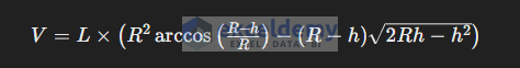
Where:
V is the volume in liters,
L is the length of the cylinder in meters,
R is the radius of the cylinder in meters,
h is the height of the liquid level in meters.
Given the specific dimensions:
L=5.0 meters (500 cm),
R=1.0 meter (100 cm),
h varies from 0.01 meters (1 cm) to 2.0 meters (200 cm)
This formula calculates the volume of the liquid based on the height from the base up to the liquid level within a horizontal cylindrical tank. To use this formula, ensure to convert all measurements (radius, length, and height) to meters before applying them in the calculation.
At 1 cm height: Approximately 9.41 liters
At 2 cm height: Approximately 26.59 liters
At 3 cm height: Approximately 48.77 liters
At 4 cm height: Approximately 74.97 liters
At 5 cm height: Approximately 104.62 liters
At 10 cm height: Approximately 293.63 liters
———————————————————
To see the full list of calculated volumes for each centimeter increment from 1 cm to 100 cm for the horizontal cylindrical tank, Download the Excel File.
List of Calculated Volumes.xlsx
Regards
ExcelDemy
Dear Curt,
It’s glad to hear that our article solved your issue. You are most welcome.
Regards
ExcelDemy
Hello Kevin,
Here the needle is pointing at 45 but as we kept the number inside the pie chart may seem 55 but actual point is 45. For your better understanding I am attaching another article for the clear view. Sorry for the confusion.
Please read this article from step 6: How to Create a Gauge Chart in Excel (With Easy Steps)
You can watch these two images to clear the confusion.
Regards
ExcelDemy
Hello Harry Ingram,
You can use this formula to extract only the numbers, including the decimal point.
=TEXTJOIN(“”, TRUE, IFERROR(IF(ISNUMBER(SEARCH(MID(B5, ROW(INDIRECT(“1:” & LEN(B5))), 1), {“0″,”1″,”2″,”3″,”4″,”5″,”6″,”7″,”8″,”9″,”.”})), MID(B5, ROW(INDIRECT(“1:” & LEN(B5))), 1), “”), “”))
Feel free to download the Excel file from the link below, you’ll find examples of the formula.
Excel file: Extract Decimal Point Numbers
Regards,
ExcelDemy
Hello Paresh Kanti Paul,
This article includes two dynamic ways for currency conversion.
Real Time Currency Converter in Excel
Regards
ExcelDemy
Hello Martin,
We are glad to hear that you found this article useful! Including a real-life example in tutorials can indeed make the steps more relatable and easier to understand. Applying these models to specific scenarios like maximizing profit by determining the production units for products A and B is a great way to leverage linear programming. We will include this in our next update.
Regards
ExcelDemy
Hello Karunesh Pandey,
As calibration details varies with lab type we can provide you the criteria. You can fill out your information and edit the list.
Regards
ExcelDemy
Hello Gary Ward,
Thanks for your valuable suggestion we will include this in our article.
Regards
ExcelDemy
Hello Liz,
You can avoid the absolute reference ($ sign). Here absolute reference is used so that it can avoid error if anyone copy the formula in another cell.
Regards
ExcelDemy
Hello Alphonse,
We are glad to hear from you again! Don’t worry about missed message, technical glitches happen to the best of us. We are glad to hear that the code for counting Mondays worked well for you. Thank you so much for expressing your gratitude—it’s always means a lot to us to know when something was helpful. You are most welcome and cheers to you too.
Regards
ExcelDemy
Hello Cynthia Satterwhite,
Neither any problem nor any solution are given. These dataset are given to practice by yourself.
Regards
ExcelDemy
Hello Nilanjan,
Excel for Mac doesn’t support the WorksheetFunction.WebService method due to differences in how Excel for Mac interacts with web services compared to Excel for Windows. In Mac, you need to directly access Google Translate’s API using HTTP requests or using a different method provided by Google Translate.
Replace “YOUR_API_KEY” with your actual Google Cloud Platform API key.
Remember to enable the “Microsoft XML, v6.0” reference in the VBA editor (under Tools > References) to use CreateObject(“MSXML2.XMLHTTP”) for making HTTP requests.
Regards
ExcelDemy
Hello Umang,
Here are some articles from where you can download dataset of different types to practice your skills.
Excel Sample Data (Free Download 13 Sample Datasets)
Excel Data for Analysis (Free Download 11 Suitable Datasets)
Excel Data for Practice Free Download
Regards
ExcelDemy
Hello Sameul Smith,
You can follow any of the methods of your choice to make your list. If you face any problem regarding it you can share your list with us. If you want to upload any image or Excel file you can post it on our ExcelDemy Forum.
Regards
ExcelDemy
Hello Fredrick Aringo,
You must use the last line to do AutoFilter based on criteria.
Please avoid the first line. We updated our code.
Regards
ExcelDemy
Dear Bharath L,
You are most welcome. We are glad that our solution worked for you.
Regards
ExcelDemy
Hello,
These datasets are given to use it for practice purpose. Currently we don’t have any solution of the task. But if you want you can send your completed task, we will review it for you.
Regards
ExcelDemy
Hello NadineB,
You are most welcome. Thanks a lot for your appreciation.
Regards
ExcelDemy
Hello Valen,
Can you mention the URL, please? In our site all URL’s of this article are working perfectly.
Regards
ExcelDemy
Hello Dianne Waginauru,
You are most welcome and thanks for your appreciation. All the very best for you project management journey.
Regards
ExcelDemy
Hello Gwenn,
Thanks for your suggestion. We deeply appreciate the solution provided in the comments. Thank you for your helpful contribution!
Regards
ExcelDemy
Hello Ameer Ahmed,
We don’t have any dataset you asked for and your question is not clear enough. Our datasets are given in the article.
Regards
ExcelDemy
Hello Gaurav,
You are most welcome.
Regards
ExcelDemy
Hello Joellah,
Thanks for your appreciation, it means a lot to us. We are trying our best to provide Excellent articles. Keep reading to boost your knowledge.
Regards
ExcelDemy
Hello Leonardo Lagos,
You can use the HYPERLINK function in Excel 360 online version.
Insert the following formula in your formula bar: =HYPERLINK(“#’SheetName’!A1”, “Link Text”)
But unfortunately, you can’t directly use the context menu to add a hyperlink to another sheet in Excel Online. You’ll need to use the formula approach described above.
Regards
ExcelDemy
Hello Shaul Bel,
Thanks for your appreciation. You’re welcome and I’m really glad to hear that the SUBTOTAL formula worked well for you in achieving the desired results. If you have any more questions or need further assistance with formulas or anything else, feel free to ask!
Regards
ExcelDemy
Hello Michelle G,
Thank you for reaching out to us. We request your attention to the above article to get your desired template on bonds purchased at a discount using the effective interest rate method.
Your requested update is incorporated into our template. Please refer to the sheet named ‘Effective Interest (Discount)’ for the template on bonds purchased at a discount using the effective interest rate method. Click on the three dots (…) if you don’t find the template in your downloaded file.
Regards
ExcelDemy
Hello Martin,
Excel for Mac does not offer right-clicking option like Excel for Windows.
You can double click on the macro button or you can try the control click.
A common workaround is to delete the existing button and create a new one, typing the correct text when you first insert it. While this might seem inefficient but you can “edit” the button text.
Regards
ExcelDemy
Hello ScubaCamper,
Thanks for your appreciation. You are getting the error with asterisk because your formula attempts to multiply by 1 (*1) directly within the MID function’s parameters, that is not correct. You need to apply the multiplication outside of the MID function but within the array operation.
Please try this formula:
=TEXTJOIN(“”, TRUE, IFERROR(MID(B5, ROW(INDIRECT(“1:” & LEN(B5))), 1)* 1, “”))
In your formula style the formula would be: textjoin(“”,true,iferror((mid([cellref],row(indirect(“1:”&LEN([cellref]))),1)*1),””))
The purpose of multiplying by 1 (*1) in Excel formulas often is to convert text numbers to actual numeric values.
Regards
ExcelDemy
Hello Dan,
You can use this VBA code to delete sheet named “BETA”, from multiple Excel files which are in same folder.
Regards
ExcelDemy
Hello Michelle,
You are most welcome. Your appreciation means a lot to us.
Regards
ExcelDemy
Hello Terry Wayne Sutfin,
Thanks for your appreciation, it means a lot to us.
Regards
ExcelDemy
Hello Margit,
You are most welcome.
Regards
ExcelDemy
Hello Jitendra Sahu,
Thanks for your kind words. Our goal is to make Excel easy for everyone.
Regards
ExcelDemy
Hello Melissa,
We are glad that our article solved your problem. You are most welcome. Thanks for your appreciation.
Regards
ExcelDemy
Hello Robert,
You are most welcome. Thanks for your appreciation.
Regards
ExcelDemy
Hello Ayokanmi,
Thanks for your appreciation. You are most welcome. Our paid courses are in Udemy not in WordPress. But we have 7500++ free tutorials and 340+ YouTube videos. You can explore these learning materials for free.
Regards
ExcelDemy
Hello Feven,
You are most welcome.
Regards
ExcelDemy
Hello Brent Hamilton,
Thank you for your feedback. We used Microsoft 365 at work. We apologize for any confusion caused. The reason the “Show Changes” feature only becomes available after saving the file on OneDrive for real-time collaboration and tracking of changes. If you save it on OneDrive, it allows Excel to track changes made by different users and enables the “Show Changes” feature to display those revisions. This integration with OneDrive enhances collaboration and ensures that users can effectively manage changes made to shared documents.
Regards
ExcelDemy
Hello David Rascati,
You are most welcome. If you want you can share your code here so that we can debug it to find out the reason.
Regards
ExcelDemy
Hello Mervyn,
Thanks for visiting our blog and sharing your questions. You wanted to clarify the difference between a Table and a Dynamic Table.
Table and Dynamic table may look similar but they are not same.
In the context of the article,
Regular Table – is created manually by the user within Excel’s interface.
Dynamic Table – is generated automatically using VBA code.
When data is turned into a table, Excel automatically adds functions like sorting, filtering, and structured referencing. These tables are dynamic and adjust automatically when the data changes.
But a Dynamic Table in the article’s context likely refers to a table created dynamically using VBA code from a range. It is able to automatically manage specific criteria or changes.
Regards
ExcelDemy
Hello Phil Hall,
If you want the Excel Workbook of this article you will get it from Download Practice Workbook section.
If you want the get the advanced exercises from “Get FREE Advanced Excel Exercises with Solutions!” button please fill your information correctly in the form. Next, you will get the exercise list in your given email. For your concern I tried it again it’s working perfectly.
Regards
ExcelDemy
Hello Vijay,
Thanks for your appreciation.
Regards
ExcelDemy
Dear RB,
You are most welcome.
Regards
ExcelDemy
Dear SKM,
You are most welcome.
Regards
ExcelDemy
Dear Sudarshan Dhuru,
You are most welcome. Thanks for your appreciation it means a lot to us.
Regards
ExcelDemy
Dear Xyand,
You are most welcome. Thanks for appreciation. We updated the image of Method 6.
Regards
ExcelDemy
Hello Saeed Anwar,
You can download the Cheat Sheet free of cost just by providing your valid email address. To get the files go to the “Download Excel Formulas Cheat Sheet PDF & Excel Files” section of this post and enter your email address. Then check your email immediately after to get the download links.
Best Regards
ExcelDemy
Hello Minzameera,
Hope you are doing well. Here we calculated the overtime based on your criteria. We assumed that this time spans are for one person. If these are for different person you can modify the formula.
Formula ta calculate working hours: =(IF(B2
Formula to calculate the total working hours: =C2+C3
Formula to calculate the overtime, here we assumed the working hours are 8: =IF(D2>B6,D2-B6,”No Overtime”)
Regards
ExcelDemy
Hi Paulinus Friday,
You are most welcome. Data Files are available in the Excel Practice file section.
Regards
ExcelDemy
Hello ابو معاذ,
You are most welcome.
Regards
ExcelDemy
Hello Dwbi,
You are most welcome.
Regards
ExcelDemy
Hello Rao,
We will try to upload it in our up coming videos.
Regards
ExcelDemy
Hello Jessica H,
You are most welcome.
Regards
ExcelDemy
Hello Jennifer,
You are most welcome.
Regards
ExcelDemy
Hello Federico Cofederi,
To send Email without pressing “Send” you can use .Send property in your code instead of .Display.
Regards
ExcelDemy
Hello Obinna,
You are most welcome.
Regards
ExcelDemy
Hello Prakash,
You are most welcome.
Regards
ExcelDemy
Hello Salomé Magerstein,
You are most welcome.
Regards
ExcelDemy
Hello Kristi,
You are most welcome.
Regards
ExcelDemy
Hello Muhammad Ismail Jumarang,
You are most welcome.
Regards
ExcelDemy
Hello Lory,
You can use the following formula: =IFERROR(INDEX(‘Round 1′!$B$3:$AJ$25,MATCH(A5,’Round 1’!$B$3:$B$25, 0),34),””)
It will leave a cell blank if no matches are found.
Regards
ExcelDemy
Hello Kndn,
The Measuring unit of the result is “Mile”.
Hello,
You are most welcome.
Regards
ExcelDemy
Hello,
You are welcome.
Regards
ExcelDemy
Dear Icarus Builders,
You are most welcome.
Regards
ExcelDemy
Hello Vini,
Updated the code spilt data into multiple Excel file.
Regards
ExcelDemy
Hello Syed Mohisn Ahmed,
Updated the code in the marked section. Where I replaced “Rupees” text from condition.
You can use the following code.
Regards
ExcelDemy
Hello,
Thanks for reaching out to us.
First, remember that rules and instructions for interest calculation after garnishment order vary among countries and states. Next, post-judgment interest accrues only on the unpaid balance of the judgment.
However, to calculate interest if the judgment was turned into a garnishment, you can follow the steps below.
1. Take your judgment amount and deduct the amount of garnishment.
2. Multiply it by your post-judgment rate (%).
3. Take the total and divide it by 365 (the number of days in a year).
4. With the amount of post-judgment interest per day (in step 3), multiply it by the number of days from your date of judgment to the date you file your execution.
Simply, use the following formula to calculate interest if the judgment was turned into a garnishment:
Interest after Garnishment = (Judgment Amount – Garnished Amount) ( Interest Rate / 365) Interim Days
Thanks again for your thoughtful comments, especially the points you made about garnishment. It adds valuable perspective to our discussion.
Regards,
Abdullah Al Masud,
ExcelDemy Team
Hello Muhammad Asif,
You are most welcome.
Regards
ExcelDemy
Hello Joseph Jabatie,
You are welcome. You can get the notes or Excel workbook from the Download section.
Regards
ExcelDemy
Hello Mohammed.
Thanks for your appreciation. Our content is completely free for our users learning but don’t use it for your business purpose without proper agreement.
Regards
ExcelDemy
Hello Mohamed Sufi,
You are most welcome.
Regards
ExcelDemy
Hello Jude Ranby,
Here, the first methods Linking Existing Table on Another Sheet in Excel is duplicating the source table.
Here, I’m attaching a video for understanding.
Regards
ExcelDemy
Hello Drishti,
Here are some article you will find more exercises.
Excel Practice Exercises PDF with Answers
Sample Excel File with Employee Data for Practice
Advanced Excel Exercises with Solutions PDF
Regards
ExcelDemy
Hello Smn,
Formula of Exercise -5: =AND(G102=”Astro”,OR(C102=”Laptop”,C102=”Mobile Phone”)) is used to check multiple conditions using the AND and OR logical functions.
Here,
G102=”Astro”: It checks the value of G102 is equal to “Astro” or not.
OR(C102=”Laptop”,C102=”Mobile Phone”): It checks the value of cell C102 is equal to either “Laptop” or “Mobile Phone”. Here, the OR function will return TRUE if any of the conditions are TRUE.
AND(G102=”Astro”, OR(C102=”Laptop”, C102=”Mobile Phone”)): Here, the AND function combines the two conditions. It will return TRUE only if both/two conditions are TRUE.
Regards
ExcelDemy
Hello M-curious,
To do a conditional formatting follow the steps of method 1. Instead of using custom option from format cells, you can use the Alignment options.
Go to Format cells dialog box then from Alignment select any select any Alignments of your choice.
Regards
ExcelDemy
Hello Dear,
You can download the Cheat Sheet free of cost just by providing your valid email address. To get the files go to the “Download Excel Formulas Cheat Sheet PDF & Excel Files” section of this post and enter your email address. Then check your email immediately after to get the download links.
Best Regards
ExcelDemy
Dear Anthonia Aniekule,
You are most welcome.
Regards
ExcelDemy
Hello Bob Leslie,
You will get Break Even Analysis Template template in this article.
Regards
ExcelDemy
Hello Oscar,
Glad to hear that our blogs are helping professionals.
Regards
ExcelDemy
Hello IDD,
If you want real-time synchronization between the Excel file on your computer and Google Sheets, you can use the Google Drive desktop app.
1. Download and install the Google Drive app on your computer.
2. Sign in with the same Google account used to upload the Excel file.
3. Copy or move the Excel file to the Google Drive folder on your computer.
Open the Excel file from the Desktop App of Drive. Then, any changes made to the file on your computer will be automatically synced with Google Drive, and subsequently, with Google Sheets.
Finally, open the google sheets from the Drive. You will get the updated Excel file.
Regards
ExcelDemy
Dear Tony
You are most welcome.
Regards
ExcelDemy
Dear Yasin,
You are most welcome.
Regards
ExcelDemy
Dear OppaPanda,
You are most welcome.
Regards
ExcelDemy
Hello Thomas,
Thanks for your appreciation. We are working on it.
Regards
ExcelDemy
Dear AKhtar Khilji,
I hope this message finds you well too. Thank you very much for your kind words and your interest in using the training material from my blog for your nonprofit Excel training program. I’m thrilled to hear that you found the content helpful and that it will be used to empower the youth of marginalized communities in Pakistan.
I’m more than happy to grant you permission to utilize the exercises from the blog for your educational initiative. Please feel free to mention “ExcelDemy” along with the web address to provide proper attribution. It’s wonderful to know that the material will be shared with the trainees to enhance their learning experience.
If you have any specific requests or need further assistance with anything related to the training material, please don’t hesitate to reach out. I’m here to support your efforts in any way I can.
Wishing you great success with your Excel training program and the empowerment of the youth in marginalized communities.
Best regards,
ExcelDemy
Hello Rahul,
You are most welcome.
Regards
ExcelDemy
Hello AJ,
You are most welcome.
Regards
ExcelDemy
Hello Ankur Vaish,
Thanks for your suggestions.
Hello Sam Arthur,
You are most welcome.
Regards
ExcelDemy
Dear John Summers,
You are most welcome. Your appreciation means a lot to us to write such technical and informative article in future.
Regards
ExcelDemy
Hello Tiffany A Snyder,
You are most welcome.
Regards
ExcelDemy
Hello Earlington Etienne,
You are most welcome.
Regards
ExcelDemy
Hello Loni,
You are most welcome.
Regards
ExcelDemy
Hello,
You are most welcome.
Regards
ExcelDemy
Hello Jane Wanjiku,
You are most welcome.
Regards
ExcelDemy
Hello Sandra Merlo,
You are most welcome.
Regards
ExcelDemy
Hello Gallienus,
You are most welcome.
Regards
ExcelDemy
Hello John,
You are most welcome.
Regards
ExcelDemy
Dear Margaret,
You are welcome.
Regards
ExcelDemy
Hello Akram Siddique,
Here, in the formula : =WEEKDAY(B5,11)
11 means – Numbers 1 (Monday) through 7 (Sunday). Here the weeks starts from Monday. So it will count the days of week from Monday and the integer value will be 1, Tuesday (2) and so on.
Regards
ExcelDemy
Hello Noelle,
To highlight the entire row, insert the following formula: =$C5 < TODAY()
In applies to select the rows
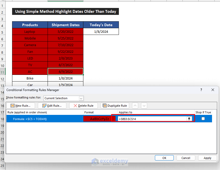
Regards
ExcelDemy
Dear Daniela Vognar,
You are most welcome.
Regards
ExcelDemy
Dear Radu Pescaru,
Sunteți foarte bineveniți.
Regards
ExcelDemy
Hello Patricia Pearson,
You are most welcome.
Regards
ExcelDemy
Hello Ehia,
You are most welcome.
Regards
ExcelDemy
Hello
You are most welcome.
Regards
ExcelDemy
Hello Chris,
You are most welcome.
Regards
ExcelDemy
Hello Sirajudeen,
You are most welcome.
Regards
ExcelDemy
Hello Patrick Opiola,
Thanks for your appreciation.
Regards
ExcelDemy
Hello Mardell Daubney,
Thanks for your appreciation.
Regards
ExcelDemy
Hello Dr.M. Veerendra Kumar,
You are most welcome.
Regards
ExcelDemy
Hello Hamed,
You are most welcome.
Regards
ExcelDemy
Hello AJ,
You are most welcome.
Regards
ExcelDemy
Hello Joedel,
You are most welcome.
Regards
ExcelDemy
Hello Abdul Kader Osman,
You are most welcome.
Regards
ExcelDemy
Dear Saiful Amin,
You are most welcome.
Regards
ExcelDemy
Hello Abdrman,
You are most welcome.
Regards
ExcelDemy
Hello Nick,
You are most welcome.
Regards
ExcelDemy
Hello Gianluigi,
You are most welcome.
Regards
ExcelDemy
Hello JC,
You are most welcome.
Regards
ExcelDemy
Hello JC,
You are most welcome.
Regards
ExcelDemy
Hello Andrii,
You are welcome.
Regards
ExcelDemy
Hello Syed Minhaj,
You are most welcome.
Regards
ExcelDemy
Hello Peter,
So kind of you.
Regards
ExcelDemy
Hello Nurit,
You are most welcome.
Regards
ExcelDemy
Hello Ava,
Thanks
Hello Tamiko,
You are most welcome.
Regards
ExcelDemy
Hello Huongpt,
You are welcome.
Regards
ExcelDemy
Hello Brenda Gale Austin-Sanders,
You are most welcome.
Regards
ExcelDemy
Dear Mario,
You are most welcome.
Regards
ExcelDemy
Hello Amanz,
We shared our ideas with you in your ExcelDemy Forum post.
Hello Adam Ingleton,
You are most welcome.
Regards
ExcelDemy
Hello Ani,
You are most welcome.
Regards
ExcelDemy
Hello Vijiaselvam Nayagam,
You are most welcome.
Regards
ExcelDemy
Hello Mohammad,
You are welcome.
Regards
ExcelDemy
Hello Suzie,
Glad to hear that our solution helped you.
Regards
ExcelDemy
Hello Romeo Nyi,
You are most welcome.
Regards
ExcelDemy
Dear Minzitia Lawrence,
You are welcome.
Regards
ExcelDemy
Hello Juan,
You are most welcome.
Regards
ExcelDemy
Dear Kagiso,
Thanks for your appreciation.
Regards
ExcelDemy
Hello Azreim,
You are most welcome.
Regards
ExcelDemy
Thanks for your appreciation.
Regards
ExcelDemy
Hello Lee G,
You are most welcome.
Regards
ExcelDemy
Hello Tanveer,
Thanks for your appreciation.
Regards
ExcelDemy
Hello Mian Muhammad Saleem,
You are most welcome.
Regards
ExcelDemy
Hello JD,
You are most welcome.
Regards
ExcelDemy
Hello Eduardo,
You are welcome.
Regards
ExcelDemy
Dear Sam,
Thanks for your appreciation.
Regards
ExcelDemy
Hello Mongwongprue Marma,
You are welcome.
Regards
ExcelDemy
Hello Calin,
You are most welcome.
Regards
ExcelDemy
Hello Adam,
Thanks for your appreciation. You are most welcome.
Regards
ExcelDemy
Hello Ali,
Thanks for your appreciation. You are most welcome.
Regards
ExcelDemy
Hello Dawood,
Thanks for your appreciation.
Regards
ExcelDemy
Hello Eduardo,
Kindly share your Excel File and images in ExcelDemy Forum.
Regards
ExcelDemy
Hello Daniel Woods,
To make problem sharing easier we launched ExcelDemy Forum, so that you can upload Excel Files and images of your problem. You can share your workbook in ExcelDemy Forum our expert team will reach out to you.
Regards
ExcelDemy
Hello Daniel Woods,
To make problem sharing easier we launched ExcelDemy Forum, so that you can upload Excel Files and images of your problem. You can share your workbook in ExcelDemy Forum our expert team will reach out to you.
Regards
ExcelDemy
Hello Abishek,
You are most welcome.
Regards
ExcelDemy
Hello David,
Thanks for your valuable suggestions.
Regards
ExcelDemy
Hello Mike Longoria,
You are most welcome.
Regards
ExcelDemy
Hello Z Thomas,
You are most welcome.
Regards
ExcelDemy
Dear Andrija,
You are most welcome.
Regards
ExcelDemy
Hello Mohammed,
Kindly share the issues you are facing while using the Excel file in the comment box. In case you need to share images, Excel file, you also can post your problem in ExcelDemy Forum.
Regards
ExcelDemy
Hello Syifaa’ Mustafa,
To get the Developer tab follow the steps mentioned in the article “Display the Developer tab in Excel“. Then you can use it to create Tooltip.
Regards
ExcelDemy
Hello Selam,
You are most welcome.
Regards
ExcelDemy
Hello DanJ,
You are most welcome.
Regards
ExcelDemy
Hello Matt S,
You are most welcome.
Regards
ExcelDemy
Hello Odedele Olufemi,
You are welcome.
Regards
ExcelDemy
Hello Joel,
You are most welcome.
Regards
ExcelDemy
Hello Chanyalew,
Thanks for your appreciation.
Regards
ExcelDemy
Hello Lynn,
You are most welcome.
Regards
ExcelDemy
Hello Nasir Ahmed,
Thanks for your appreciation.
Regards
ExcelDemy
Dear Anon,
You are most welcome.
Regards
ExcelDemy
Hello Vickie Addo,
We have given the answers of 100 questions in our Excel File, which is given in the Download Practice Workbook Section. As these questions are given to test your skills it won’t be helpful to check the answer immediately. A gif is given how you can test your skills at the end. Please download the Excel File and test you skills then see the answers.
Regards
ExcelDemy
Hello Venkatesh,
You are most welcome.
Regards
ExcelDemy
Dear Alexandar P,
You are most welcome.
Regards
ExcelDemy
Hello Naziom,
You are most welcome.
Regards
ExcelDemy
Hello Viraltecho,
You are most welcome.
Regards
ExcelDemy
Hello Joel,
You are most welcome.
Regards
ExcelDemy
Hello,
You are most welcome.
Regards
ExcelDemy
Hello Suhaili,
You don’t need to worry about payment. If you want any read-to-use template kindly send your requirements using [email protected] email.
Regards
ExcelDemy
Dear Dave,
You are most welcome.
Regards
ExcelDemy
Dear Komal Thakur,
You are most welcome.
Regards
ExcelDemy
Hello Samia,
In the Download Practice Workbook section, you will get the dataset used in the article.
Regards
ExcelDemy
Hello Nafez,
You are most welcome and thanks for you invitation to visit Qatar.
Regards
ExcelDemy
Hello May,
The “Developer Tab” option is missing in default Excel versions. You can enable it from Excel Options. By following this article Display the Developer Tab you can enable it easily.
Regards
ExcelDemy
Dear Laurie,
You are most welcome.
Regards
ExcelDemy
Dear Sovereign,
Thanks for your appreciation.
Regards
ExcelDemy
Hello Sagar,
You will get the solutions in the Excel file, which is given in the Download Practice workbook Section.
Regards
ExcelDemy
Dear Anusha Uppuganti,
You are most welcome. We are so glad that our article explanation helped you.
Regards
ExcelDemy
Dear PK,
Thanks for your appreciation. You are most welcome.
Regards
ExcelDemy
Hello Tsegay Gebreselasie,
Our aim is giving you the best Excel-related content like this.
Regards
ExcelDemy
Dear Mark,
Thanks for your appreciation.
Regards
ExcelDemy
Hello Rolan,
Thanks for your suggestion. Article is updated.
Hello Damien,
From our Download Practice Workbook section, you will get the Excel file.
If you face any difficulties after downloading the above file, follow this article to Enable Macros but Not Working
Regards
ExcelDemy
Hello Taiwo,
All the solution are available in the Excel Practice file section.
We used this formula to get discount amount: =F5*IF(D5<1,0.03,0.05)
Regards
ExcelDemy
Hi viralTecho
Thanks for your appreciation.
Regards
ExcelDemy
Hello James Ward,
To run the code from Excel you can follow these steps:
Developer tab >> Macros >> Select any Sub Procedure from the list
Regards
ExcelDemy
Hello Hugh Richards,
Thanks for your appreciation.
Regards
ExcelDemy
Dear Noe Albarran,
You are most welcome.
Regards
ExcelDEmy
Dear Yuan,
Thanks for the suggestions. The code is updated you can check it now.
Regards
ExcelDemy
Dear Amir
You have to use either the combined formula or the vba code. Because converting number to words maintaing the place vaule is not possible by simple formula.
Regards
ExcelDemy
Dear Ian Fisher,
You are most welcome.
Regards
ExcelDemy
Hello Viraltecho,
You are most welcome.
Regards
ExcelDemy
Hello Viraltecho,
You are most welcome.
Regards
ExcelDemy
Dear Roberto,
You are most welcome.
Regards
ExcelDemy
Dear Aubrey
You are most welcome. Your appreciation means a lot to us.
Regards
ExcelDemy
Dear Dilip Paunikar
You are most welcome.
Regards
ExcelDemy
Dear Soumendra
You are most welcome.
Regards
ExcelDemy
Hello Manwesh,
You can state your problem in the comment section or in our ExcelDemy Forum.
Regards
ExcelDemy
Dear Ashab,
We do have a YouTube channel named ExcelDemy
Regards
ExcelDemy
Dear Evangeline,
Thanks for your appreciation. Our experienced writers write these questions after doing a complete research about the topic.
Regards
ExcelDemy
Dear Jason,
You are most welcome.
Regards
ExcelDemy
Dear Ryan,
Glad to hear that our article helped you.
Regards
ExcelDemy
Dear Endashaw Balcha,
To know more about excel formula you can explore our Excel Formulas category. From here you will get practical use of different formulas in different fields.
Regards
ExcelDemy
Dear Raf,
You are most welcome.
Regards
ExcelDemy
Hello Muhammad Amin,
Good to hear that. To get more helpful contents explore our site.
Regards
ExcelDemy
Dear Jess,
Thanks for your appreciation.
Regards
ExcelDemy
Dear Jimmy,
You are most welcome.
Regards
ExcelDemy
Hello y2mate,
Thanks for your appreciation.
Regards
ExcelDemy
Dear ytMp3,
Thank you so much.
Regards
ExcelDemy
Dear Martin Carrion,
You are most welcome.
Regards
ExcelDemy
Dear Dina,
Thank you so much for your appreciation.
Regards
ExcelDemy
Dear Navini,
You are most welcome.
Regards
ExcelDemy
Dear Gopi Sahu,
Thanks for reaching out to us. You will get various types of WFM related articles here Excel Solver
If you need solution of any specific topic kindly comment down below.
Regards
ExcelDemy
Dear Justice,
You are most welcome.
Regards
ExcelDemy
Dear Merry,
You are most welcome.
Regards
ExcelDemy
Dear Karen,
You are most welcome.
Regards
ExcelDemy
Hi Putul ch. Borah,
Yes, you can do it by following the mentioned steps.
Dear Tiago,
You are most welcome.
Regards
ExcelDemy
Dera Ashok,
You are most welcome.
Regards
ExcelDemy
Dear Foysal,
You are most welcome.
Regards
ExcelDemy
Dear kinyapreen,
To get virtual lessons you can follow our youtube channel Youtube Channel
Regards
ExcelDemy
Hello BART,
It is possible to add a VB line of code to run the selection change code only when you click the tab of the worksheet called “index.” To achieve this, you can use the Worksheet_Activate event in the code module of the “index” worksheet. Here’s the code.
Regards
Alif Bin Hussain
Dear,
You are most welcome.
Regards
ExcelDemy
Dear Bart,
You are most welcome. Sure, you can inform us.
Regards
ExcelDemy
Dear Najeeburk,
You are most welcome.
Regards
ExcelDemy
Dear Danny Van Straten,
If you need any types of customized templates you may contact us through [email protected]
We have a expert team to create any types of professional templates.
Regards
ExcelDemy
Hello Yaojm,
Thanks for your suggestions. Here we focused on the comparison/difference of VLOOKUP and XLOOKUPp that’s why we didn’t improvised the use of VLOOKUP.
Regards
ExcelDemy
Hello Pankaj,
You are welcome.
Regards
ExcelDemy
Dear Charlotte,
You are most welcome.
Regards
ExcelDemy
Dear Mustafa,
You are most welcome.
Regards
ExcelDemy
Hello Abubakar,
You are most welcome. We hope so you will be able to create an interim certificate template following these steps.
Regards
ExcelDemy
Dear B,
You are welcome.
Regards
ExcelDemy
Dear Akash,
You are most welcome.
Regards
ExcelDemy
Dear Carl,
You are most welcome.
Regards
ExcelDemy
Hello Dear,
You can download the Cheat Sheet free of cost just by providing your valid email address. To get the files go to the “Download Excel Formulas Cheat Sheet PDF & Excel Files” section of this post and enter your email address. Then check your email immediately after to get the download links.
Best Regards
ExcelDemy
Dear Macel Williams,
To customize any templates you can contact with us via this mail problem @exceldemy.com
Regards
ExcelDemy
Dear Macel Williams,
To customize any templates you can contact with us via this mail problem @exceldemy.com
Regards
ExcelDemy
Dear Qasim,
Thanks for your suggestions we have updated our Exercise 3 you can check it now.
Regards
ExcelDemy
Dear Kenny H,
This Email address is valid but if you face any problem you can post your problem in our ExcelDemy Forum.
Regards
ExcelDemy
Dear Nikhil Pandey,
You will get all the solutions in the workbook’s Solution sheet. Here I’m giving you the query answer for your understanding.
The Formula is : =WEEKDAY(B5,11)
Regards
ExcelDemy
Dear Nikhil Pandey,
You will get the solution sheet in the Download Practice Files section. Download the workbook there in Solution sheet you will get all the solutions. You you can get the workbook from this link Solution Sheet
Regards
ExcelDemy
Dear Aiden,
Yes you can do that.
Regards
ExcelDemy
Dear Macel,
You are welcome.
Regards
ExcelDemy
Dear Marc,
You are welcome.
Regards
ExcelDemy
Dear Kim,
Thanks for your appreciation.
Regards
ExcelDemy
Dear Prakash Tulsiani,
You are most welcome.
Regards
ExcelDemy
Dear Kay,
To get a customized templates you can contact with us through this Email: [email protected]
Regards
ExcelDemy
Hello Dear,
You can download the Excel and PDF files free of cost just by providing your valid email address. To get the files go to the “Download Excel Formulas Cheat Sheet PDF & Excel Files” section of this post and enter your email address. Then check your email immediately after to get the download links.
Best Regards
ExcelDemy
Dear Nadew w/yesus,
You are most welcome.
Regards
ExcelDemy
Dear Dr,
You are most welcome.
Regards
ExcelDemy
Dear Adil Ahmed,
You are most welcome.
Regards
ExcelDemy
Dear Macel Williams,
You are most welcome.
Regards
ExcelDemy
Hello Dear,
You can download the Cheat Sheet free of cost just by providing your valid email address. To get the files go to the “Download Excel Formulas Cheat Sheet PDF & Excel Files” section of this post and enter your email address. Then check your email immediately after to get the download links.
Best Regards
ExcelDemy
Dear Isaac,
You are most welcome.
Regards
ExcelDemy
Dear MADI,
Thank you for following our article.
To split into sheets based on certain row conditions, we have to enter an IF condition that checks if the row is of a certain colour. Here, I have added the code to do this.
This code checks if the interior colour of the first cell in each row of the selected range is Green(RGB(0,255,0)). The entire row is copied and pasted into a new sheet if rows meet the condition. You can alter this colour condition according to your need.
Regards
Priti
Dear Sara,
You will find the solutions in the Excel file which is given in Download Practice Workbook section.
Regards
ExcelDemy
Dear Sakshi,
You are most welcome.
Regards
ExcelDemy
Dear Md. Morshed Alam,
You are most welcome.
Regards
ExcelDemy
Dear Alex,
Thanks for your feedback.
Regards
Exceldemy
Dear Paresh Kanti Paul,
We are glad to hear that.
Regards
ExcelDemy
Hello Dear,
You can download the Excel and PDF files free of cost just by providing your valid email address. To get the files go to the “Download Excel Formulas Cheat Sheet PDF & Excel Files” section of this post and enter your email address. Then check your email immediately after to get the download links.
Best Regards
ExcelDemy
Dear Sushil,
You are most welcome.
Regards
ExcelDemy
Dear Duncan R Walk,
You are most welcome.
Regards
ExcelDemy
Dear Bolajoko Olufemi,
You will get all resources related to Data Analysis here All About Data Analysis. We are planning to launch courses as soon as possible.
Regards
ExcelDemy
Dear Ronald,
You are most welcome.
Regards
ExcelDemy
Dear Ronhat Minmin,
If you want to get the Excel File, you can download it from Download Practice Workbook
Regards
ExcelDemy
Dear Ebrahim Ahmadi,
You are welcome.
Regards
ExcelDemy
Hello Dear,
You can download the Excel and PDF files free of cost just by providing your valid email address. To get the files go to the “Download Excel Formulas Cheat Sheet PDF & Excel Files” section of this post and enter your email address. Then check your email immediately after to get the download links.
Best Regards
ExcelDemy
Dear Lin Giralt,
You are most welcome.
Regards
ExcelDemy
Dear Khin Soe,
You are most welcome.
Regards
ExcelDemy
Dear Tha’ir,
You are most welcome.
Regards
ExcelDemy
Dear Mohamad,
Thanks for your appreciation
Regards
ExcelDemy
Dear Minhajul,
You are most welcome.
Regards
ExcelDemy
Dear Sandeep Bhattacharjee,
You are most welcome and thanks for your appreciation.
Regards
ExcelDemy
Hello Sujay Jain,
You can download the Excel and PDF files free of cost just by providing your valid email address. To get the files go to the Top 100 MCQ of Excel section of this post and enter your email address. Then check your email immediately after to get the download links.
Best Regards
ExcelDemy
Dear S Roy,
You are most welcome.
Regards
ExcelDemy
Hi Kazem,
You are welcome.
Regards
ExcelDemy
Dear Lana,
You are most welcome.
Regards
ExcelDemy
Dear Seamus Madden,
Thanks for your appreciation.
Regards
ExcelDemy
Hi Ndonwi,
Thanks
Dera Merc,
You are most welcome.
Regards
ExcelDemy
Dear Joanna,
You are most welcome.
Regards
ExcelDemy
Dear Richard,
You are most welcome.
Regards
ExcelDemy
Dear Andrei,
These functions are available in WPS office.
Regards
ExcelDemy
Dear Kapil,
You are most welcome.
Regards
ExcelDemy
Dear Tommy Fuifui,
You are most welcome.
Regards
ExcelDemy
Dear Excel Nob,
You are most welcome.
Regards
ExcelDemy
Dear Car,
You are most welcome.
Regards
ExcelDemy
Dear Jamie,
You are most welcome.
Regards
ExcelDemy
Dear Anitelleth,
You are most welcome.
Regards
ExcelDemy
Dear Anitelleth,
You are most welcome.
Regards
ExcelDemy
Dear Kay,
You are welcome.
Regards
ExcelDemy
Dear Pirooz Rahimi,
You are most welcome and thanks for your appreciation.
Regards
ExcelDemy
Dear Abel,
Thanks for your appreciation. You are most welcome.
Regards
ExcelDemy
Dear Kh Paydar,
You are most welcome.
Regards
ExcelDemy
Dear Joris,
You are most welcome. We are glad to hear that.
Regards
ExcelDemy
Dear Raja,
You are most welcome.
Regards
ExcelDemy
Dear Kapil,
Thanks for your appreciation.
Regards
ExcelDemy
Dear Polepeddi Sasidhar,
We are glad to hear that.
Regards
ExcelDemy
Hello Silpa,
You can download the Excel and PDF files free of cost just by providing your valid email address. To get the files go to the “Download Excel Formulas Cheat Sheet PDF & Excel Files” section of this post and enter your email address. Then check your email immediately after to get the download links.
Best Regards
ExcelDemy
Dear Jidith Savidge,
You are most welcome.
Regards
ExcelDemy
Dear Ajij Nadaf,
We will love to give you suggestions. kindly share your problem.
Regards
ExcelDemy
Good day, Daniel,
The issue you’re having might be because your workbook’s data range differs from the data range specified in our code.
Change the data range according to your worksheet.
This might be the solution to your issue. I’d appreciate it if you could send me the worksheet you’re working on so that I can better understand your issue and give you an exact solution.
Regards
Sakibul Hasan Nahid | ExcelDemy Team
Hey Philip,
Thanks for your response. You can use the SORT and FILTER functions along with the LARGE function to solve your problem.
Here’s the practice sheet we used. You can check it out for a better understanding.
SORT-FILTER.xlsx
You can also check out this article for more detailed explanations.
https://www.exceldemy.com/excel-top-10-list-with-duplicates/
Regards
Hassan Shuvo| ExcelDemy Team
Hello Chandan,
Thanks for commenting. If I’m not wrong, you want to match the dataset like the one below.
Select the entire dataset without the heading then go to conditional formatting >> New Rule
Then select “Use a formula to determine which cells to format.”
In the formula bar, enter the following formula:
=AND(A3<>B3,C3<>B3)
Press OK
Here, “A3” represents the cell containing the customer name, “B3” represents the cell containing the ID name, and “C3” represents the cell containing the real name. You can adjust the cell references based on your data.
Choose the formatting option that you want to use for the highlighted rows. For example, we took light green color here for highlighting.
The final outcome will look like the image below.
I hope this answer will help you to identify matched names. Please let us know if you have any other queries. Also, you can post your Excel-related problem in ExcelDemy Forum with images or Excel workbooks.
Regards
Mizbahul Abedin | ExcelDemy Team
Dear MD. KAMAL HOSSAIN,
To obtain your required format please follow the following simple steps:
From your Excel Workbook, press ALT + F11 to open Visual Basic Editor.
Insert a module.
Paste the following code:
Now, return to your worksheet. Type in the following formula in the cell where you require the output and press Enter key.
=NumberToWords(B5) & ” Taka Only”
Here, B5 indicates the reference of the cell where you have the input number.
I hope this solution will be sufficient for your requirements. Let us know your feedback.
Regards,
ExcelDemy
Dear Rich Saunders,
Query 1: The method 7 works just fine. If you write March in F4, you will get the values for that month as well.
Query 2: The formula is universal for any Excel version. If you write the formula in any cell the formula will get you the entire row value for the name you will write in the F4 cell. For example, if you write “Nathan” in F4 cell and paste the formula in the A1 cell then the formula will write the values of the entire row( B8:D8) in the A1:A3 range.
Yes, we should have mentioned the Ctrl+Shift+Enter in the article. We will make sure of that in the next articles. As we used Microsoft 365 so it works by pressing Enter. We are sorry for that.
Regards
ExcelDemy
Dear Tudor,
Hope you are doing well. Answer of your questions are given below with explanation.
1. How can I change the month and day from English to Romanian?
Select the cell with month and date, cell C7 in our case.
Right-click with the mouse and select Format Cells.
In the Format Cells window, select Romanian (Moldova) under the Locale menu.
Then, select any type under the Type menu and click the OK button.
The month and date are changed into Romanian from English. Do the same process for cell E7.
2. If an employee works on Saturday and/or Sunday, how can I collect those weekend hours separately, in a cell?
Let’s say the first employee works on Saturday and Sunday for 5 and 6 hours respectively. He works on 4 weekends which you can see in the picture. To sum these values we’ll use the SUMIFS function.
Apply the formula in any cell where you want the weekend hours, let’s say cell AM11-
=SUMIFS($F$11:$AJ$11,$F$11:$AJ$11,"<>P",$F$11:$AJ$11,"<>A")After pressing Enter you’ll get the total weekend hours. You can use the Fill Handle tool to apply this formula to other employees.
Dear Aspen,
You are most welcome.
Regards
ExcelDemy
Thanks for your suggestions.
Dear Victor,
You are most welcome.
Regards
ExcelDemy
Dear Elizabeth,
You are most welcome. We are so glad that our article fulfilled your need.
Regards
ExcelDemy
Dear Anjli Gupta,
Answers are given in the Solution sheet of Excel File which is in Download Practice Workbook section.

Regards
ExcelDemy
Dear HG,
You are most welcome.
Regards
ExcelDemy
Dear Seaunders,
Thanks for your appreciation. It means a lot to us.
Regards
ExcelDemy
Dear Gunawan,
Thanks for your suggestions. We updated the article. You can check it now.
Regards
ExcelDemy
Hi Fake Hidden,
Thanks for your suggestions. We updated our article so that it fulfills the need of all types of readers. You may check our article now and let us know any kinds of suggestions.
Regards
ExcelDemy
Dear Rafi,
Thanks for your appreciation.
Regards
ExcelDemy
Dear Elly,
Thanks for your appreciation. We re-explained our formulas to make them more understandable. If you find any difficulty now, let us know in the comment section below.
Regards
ExcelDemy
Dear Rashmi,
You are most welcome.
Regards
ExcelDemy
Dear Jay Dee,
That’s good to hear. We are interested to know more from you.
Regards
ExcelDemy
Dear Silver,
You are most welcome.
Regards
ExcelDemy
Dear William B,
You are most welcome.
Regards
ExcelDemy
Dear Eugen Safta,
You are most welcome.
Regards
Shamima Sultana | ExcelDemy
Dear Radu,
Thanks for your suggestion and we appreciate it. We updated the cell range.
Dear Sanket,
Thanks for your appreciation.
Regards
Shamima Sultana
Project Manager | ExcelDemy
Dear Yar Zar Htun,
You are most welcome. We are glad that through ExcelDemy you are improving your skill.
Regards
Shamima Sultana
Project Manager | ExcelDemy
Dear Vivasvan,
You are most welcome. It’s great to know that our article helped you to complete your project.
Regards
Shamima Sultana
Project Manager | ExcelDemy
Dear Bo Thibaut,
We are willing to do any Excel-related projects. Kindly share your requirements through this Email: [email protected]
Regards
Shamima Sultana
Project Manager | ExcelDemy
Hi Robert Bakinam,
Here, you will get the full copy in pdf Marking Result Sheet.
Regards
Shamima Sultana
Project Manager | ExcelDemy
Dear German,
You are most welcome. To get solutions with detailed explanations, follow ExcelDemy.
Regards
Shamima Sultana
Project Manager | ExcelDemy
Dear Kirsten Wheeler,
Thanks for your appreciation. To get solutions with detailed explanations, follow ExcelDemy.
Regards
Shamima Sultana
Project Manager | ExcelDemy
Dear NancyM,
Thanks for your appreciation. To get solutions with detailed explanations, follow ExcelDemy.
Regards
Shamima Sultana
Project Manager | ExcelDemy
Dear CJvW,
Thanks for your appreciation. To get more helpful content be with ExcelDemy.
Regards
Shamima Sultana
Project Manager | ExcelDemy
Dear Geogre,
Thanks for your kind attention and suggestion. We updated it.
Dear Michael Gamal Aziz,
You are most welcome.
Regards
Shamima Sultana
Project Manager | ExcelDemy
Dear Glenn,
We are glad to hear that. ExcelDemy is trying hard to give you quality content.
Regards
Shamima Sultana
Project Manager | ExcelDemy
Dear Uday Kumar,
We are working on your problem. We will appreciate you to post your problem in our ExcelDemy Forum.
Regards
Shamima Sultana
Project Manager | ExcelDemy
Dear Ramandeep Kaur,
Thanks for your appreciation. Sooner we will make another exercise based on Basic and Advanced Formulas.
Regards
Shamima Sultana
Project Manager | ExcelDemy
Dear Datla Srinivas,
We are working on your requirements. We hope we will come back to you with your expected solutions.
Regards
Shamima Sultana
Project Manager | ExcelDemy
Dear Mody,
Thanks for your appreciation.
Regards
Shamima Sultana | Project Manager | ExcelDemy
Hello Joanie,
You are most welcome.
Regards
Shamima Sultana | Project Manager | ExcelDemy
Dear Map,
Thanks for your appreciation and suggestion. Sooner we will write an article regarding this topic.
Regards
Shamima Sultana | Project Manager | ExcelDemy
Dear Ven Upekkha,
Thanks for your appreciation.
Regards
Shamima Sultana | Project Manager | ExcelDemy
Dear Rajesh,
You are welcome.
Regards
Shamima Sultana | Project Manager | ExcelDemy
Dear umit,
Thanks for your appreciation it means a lot to us.
Regards
Shamima Sultana | Project Manager | ExcelDemy
Hello Zuri,
Thanks for your suggestion.
Regards
Shamima Sultana | Project Manager | ExcelDemy
Dear Carl,
Thanks for your appreciation. ExcelDemy is glad to help you.
Regards
Shamima Sultana | Project Manager | ExcelDemy
Dear Sandra Aldridge,
Thanks for your appreciation it means a lot to us. ExcelDemy is glad to help you.
Regards
Shamima Sultana | Project Manager | ExcelDemy
Dear Micah,
Thanks for your kind words. ExcelDemy is dedicated to provide solutions to help you.
Regards
Shamima Sultana | Project Manager | ExcelDemy
Dear Mukibul Hasan,
Thanks for your appreciation. Stay in touch with ExcelDemy.
Regards
Shamima Sultana | Project Manager | ExcelDemy
Dear Shanmuga Raja V S,
Thanks for your appreciation. Stay in touch with ExcelDemy.
Regards
Shamima Sultana | Project Manager | ExcelDemy
Dear Adam,
Thanks for your appreciation.
Shamima | Project Manager | ExcelDemy
Dear Zidane,
Thanks for your appreciation.
Shamima | Project Manager | ExcelDemy
Dear Kayla,
Thanks for your appreciation and we are glad that our Dataset Template helped you.
Regards
Shamima | Project Manager | ExcelDemy
Hello Uday Kumar,
Kindly check the reply to your previous comment. We have given you a non-macro solution.
Dear Forte,
Thanks for your appreciation. Stay in touch with ExcelDemy to get more helpful content.
Regards
Shamima | Project Manager | ExcelDemy
Dear Gilson,
Thanks for your appreciation. Stay in touch with ExcelDemy to get more helpful content.
Regards
Shamima | Project Manager | ExcelDemy
Dear Gerry Conroy,
You are most welcome.
Regards
Shamima | Project Manager | ExcelDemy
Dear Syed Anwar Hussain,
Thanks for your appreciation.
Regards
Shamima | Project Manager | ExcelDemy
Hello, Xzavier!
For better understanding, we updated the article. Kindly check it now it would be helpful.
Regards
ExcelDemy
Hello, An!
You are most welcome. To get helpful content follow ExcelDemy.
Regards
ExcelDemy
Hello, James!
Your appreciation means a lot to us. To have a more wonderful experience follow ExcelDemy.
Regards
ExcelDemy
Hi Rassulsson!
Thanks for your appreciation.
Regards
ExcelDemy
Thanks, Michael, for your query. From your comment, it seems that you want to permanently assign the replacing dataset (denoted by Reprng in the code) instead of taking them in a prompted input box. You can do that by following the steps below.
1. First, set a Name to the range that contains the Find & Replace with columns (In this case E5:F6). To do that, select the range and type a suitable name on the Name Box. Suppose you give the name “Find_Replace_Array”
2. Now, open a new module and write the given code of method 1.
3. Then, on the code, replace the line :
Set Reprng = Application.InputBox(“Replace with: “, Title, Type:=8)
With the following line.
Set Reprng = Range(“Find_Replace_Array”)
Now, if you run the code, you will only need to select the range where you want to replace values and it will automatically replace the values for you. Here, you will not be required to manually input the address of Find_Replace_Array.
Hope it does the job for you. If you have any further queries, do let us know. Moreover, if your problem persists, you can post your problem in our Exceldemy Forum along with your Excel file.
Hello, Hamza!
Thanks for your appreciation. We are glad that our article helped you.
Regards
ExcelDemy
Hello, A!
If your file is protected by using Encrypt with Password feature then it won’t work. We mentioned it in the Things to Remember section.
Regards
ExcelDemy
Hello, Nabil sellami!
Thanks for your appreciation. To get more enjoyable articles stay in touch with ExcelDemy.
Regards
ExcelDemy
Hello, JeteMc!
Welcome, JeteMc. To get more helpful information stay in touch with ExcelDemy.
Regards
ExcelDemy
Hello, Helen!
Thanks for your appreciation. To get more helpful information stay in touch with ExcelDemy.
Regards
ExcelDemy
Hi, Irene!
Thanks for your appreciation. To get more helpful information stay in touch with ExcelDemy.
Regards
ExcelDemy
Hi, Elton!
Thanks for your appreciation. We will try to launch pdf files.
Regards
ExcelDemy
Hello, Muhammad Luqman!
You can download it from Download Excel Formulas Cheat Sheet PDF section.
Regards
ExcelDemy
Hi, Bosco!
Thanks for your appreciation. To get more informative contents stay in touch with ExcelDemy.
Regards
ExcelDemy
Hello, Joe Smith!
The 64-bit version of Excel is not compatible with 32-bit active x controls. To know more about it you can visit this site
Regards
ExcelDemy
Hello, Aleksandra!
Thanks for your appreciation.
Regards
ExcelDemy
Hello, Bennie!
Thanks for your appreciation.
Regards
ExcelDemy
Hello, Harry!
You can download the copy from Download Sample Workbook
Regards
ExcelDemy
Hello, Emil Lazar!
Thanks for your appreciation. Stay in touch with ExcelDemy to get more useful articles.
Regards
ExcelDemy
Hi Abishek Sharma!
If you want the Excel file then you can download it from the Download Practice Workbook section. Or you need other assistance you can comment or send us mail at [email protected]
Hello, Nastaran!
Thanks for your appreciation. We are glad that our post helped you.
Regards
ExcelDemy
Hello, Ruben!
It’s glad to know that our content is helpful to you. To know more about Excel stay in touch with ExcelDemy.
Regards
ExcelDemy
Hello, Tanael Wawe!
You are welcome. Stay in touch with ExcelDemy to get more helpful content.
Regards
ExcelDemy
Hello, Tanael Wawe!
Thanks for your appreciation. Stay in touch with ExcelDemy to get more helpful content.
Regards
ExcelDemy
Hello, Dan!
Thanks for your appreciation. It means a lot.
Regards
ExcelDemy
Hello, Ahnaf!
You are most welcome. stay in touch with ExcelDemy.
Regards
ExcelDemy
Hello, Aleem!
Thanks for your appreciation. stay in touch with ExcelDemy.
Regards
ExcelDemy
Hello, Mohan!
Thanks for your appreciation. Stay in touch with ExcelDemy for more helpful content.
Regards
ExcelDemy
Hello, Many!
You are most welcome. To get more helpful content with explanations stay in touch with ExcelDemy.
Regards
ExcelDemy
Hello, ExcelAmateur!
Thanks for your appreciation. To get more helpful content with explanations stay in touch with ExcelDemy.
Regards
ExcelDemy
Hello, Mubashir!
Thanks for your appreciation. To get more helpful content stay in touch with ExcelDemy.
Regards
ExcelDemy
Glad to hear that.
Regards
ExcelDemy
Thanks for your appreciation.
Regards
ExcelDemy
Hello!
Thanks for your appreciation.
Regards
ExcelDemy
Hello, Andy W!
Thanks for your appreciation.
Regards
ExcelDemy
Hi, Dhaval!
Thanks for your appreciation.
Regards
ExcelDemy
Hello, Pankaj!
We are glad to know that it worked for you. To get more useful content stay in touch with ExcelDemy.
Regards
ExcelDemy
Hello, Suzette!
Thanks for your appreciation. We will try to use fonts that will be easier to read for old eyes.
Regards
ExcelDemy
Hello, Eric!
Thanks for your appreciation. To get more helpful content stay in touch with ExcelDemy.
Regards
ExcelDemy
Hello, Instast!
Thanks for your appreciation. To get more helpful content stay in touch with ExcelDemy.
Regards
ExcelDemy
Greetings ASHISH PANT,
I appreciate you asking this question. We use the Microsoft Office 365 version here. In order to resolve your problem, you need to open the Excel workbook in Microsoft Office 365 version.
Regards
ExcelDemy
Hello, Andre!
Thanks for your appreciation. To get more helpful posts stay in touch with ExcelDemy.
Regards
ExcelDemy
Hello, Michelet!
Thanks for your appreciation. Stay in touch with ExcelDemy.
Regards
ExcelDemy
Hello, Im!
Hope you are doing well. Thanks for your appreciation.
Regards
ExcelDemy
Hello, Leslie!
Hope you are doing well. Thanks for your appreciation. Stay in touch with ExcelDemy.
Regards
ExcelDemy
Hello, Aston!
Hope you are doing well. To show your data labels in millions kindly follow this article Millions in Data Labels
Regards
ExcelDemy
Hello, Chan!
Hope you are doing well. Glad to know that our content is useful for you.
Regards
ExcelDemy
Hello, Kim!
Thanks for your appreciation. For more useful content visit our site ExcelDemy.
Regards
ExcelDemy
Hello, Suki Nasoordeen!
Thanks for your appreciation. Stay in touch with ExcelDemy.
Regards
ExcelDemy
Hello Gerald,
Do you need to know the conversion from Excel to PDF? Right? Because the original bank statement was in PDF format. So, here you can follow the steps below to convert your Excel file back to PDF file.
Firstly, you need to open your Excel file.
Secondly, click the File button at the top-left corner of the Excel file.
Thirdly, go to Save As and click it.
Fourthly, choose PDF from the Save option at the top-right corner by clicking the drop-down button.
Finally, choose a particular location to keep it by selecting Browse button.
Thanks
Regards
ExcelDemy
Hello, Chole Faulkner!
Thanks for your appreciation. Stay in touch with ExcelDemy.
Regards
ExcelDemy
Hello, SS!
Hope you are doing well. We are very sorry that you are facing some troubles with advertising. But will try our best to give you a nicer experience.
Regards
ExcelDemy
Hi Zidane
Hope you are doing well. Thanks for your appreciation.
Regards
ExcelDemy
Hi Peter
Thanks for your appreciation.
Regards
ExcelDemy
Hi Mohammed Hassen,
Thank you so much.
Thanks
Regards
ExcelDemy
Hi N,
Thanks for your appreciation. Please visit our site for more excel-related problems.
Thanks
Regards
ExcelDemy
Hi Bernadeth,
Thanks for your appreciation. To get more useful content kindly visit our site.
Thanks
Regards
ExcelDemy
Hi GIRIDAR N,
Thanks for your appreciation and we are glad to help you. For any types of Excel-related problems kindly reach out to us.
Regards
ExcelDemy
Hello Marian,
There are some unwanted issues that may arise while dealing with the VBA code. In that case, you need to utilize the following code.
Here, the Application path and pdf path need to be defined accurately. Then, when you run the code, you will find the copied items in the clipboard.
Then, click on Paste all to extract values.
Thanks
Author, ExcelDemy
Hi Exceler,
Here, I tried the first method for 50 sets of data and it worked but you have to change the cell references based on your dataset. For your better understanding, I am attaching the images along with the formula.
=INDEX($D$5:$D$30,MATCH(1,MMULT(--($B$5:$C$30=F5),TRANSPOSE(COLUMN($B$5:$C$30)^0)),0))The images of datasets
Here, I used the formula for the entire dataset. I changed the references based on my dataset.
Output for 50 values:
Note: If your dataset is very large kindly send us your dataset
Thanks
Shamima Sultana
Hi Tom Lynham
Hope you are doing well. Here, I updated the article which implies the title and the explanation.
By following above explained methods it is possible to print colorful gridlines but you must use a color printer.
If this update doesn’t help you or you have further queries kindly let us know.
Thanks
Shamima Sultana
Hello Mark,
We uploaded the Excel files again, you can check these files also. If you find any difficulty opening the file let us know.
Thanks
Hello Mark,
Hope you are doing well.
Whenever I try to download this workbook it works fine without a password. To be reassured a couple of my teammates also downloaded this file they also didn’t face any difficulty.
As I haven’t used any password for this worksheet. I really want to know what caused such issues while you downloaded the file.
Here, I will show you what it looks like when I download the file again.
After downloading the file Excel shows a warning message. You have to click on Enable Editing.
Later, the downloaded file will be available to use or you can make any changes you want.
N.B. If this solution doesn’t work for you. Kindly sent me the screenshots of the problem.
Thank you.
Regards
Shamima Sultana
Hi Froggy,
Hope you are doing well. Thanks for reaching out to us with your issue.
As you intend to apply the above code to a workbook with multiple sheets so you need to add some extra lines in your code to define all available worksheets or selected worksheets.
Here, I will give you two solution
1. For selected sheets
2. For all the available sheets in a workbook
1. If you want to apply the same code in some selected sheets then use the code given below where I declared sheets names by using an Array.
Option Explicit
Sub AddSpaceBetweenRows()
Dim all_sheets As Worksheet
Dim rng As Range
Dim i As Long
Dim all As Variant
Set all = sheets(Array(“VBA1”, “VBA2”))
For Each all_sheets In all
all_sheets.Select
Set rng = Range(“B5:E9”)
For i = rng.Rows.Count To 2 Step -1
rng.Rows(i).EntireRow.Insert
Next i
Next
End Sub
2. To loop through all the available sheets of your workbook you will need to use the code given below where I declared all_sheets and used an extra For Loop.
For your better understanding, I’m providing the modified code here,
Option Explicit
Sub AddSpaceBetweenRows()
Dim all_sheets As Worksheet
Dim rng As Range
Dim i As Long
For Each all_sheets In Worksheets
all_sheets.Select
Set rng = Range(“B5:E9”)
For i = rng.Rows.Count To 2 Step -1
rng.Rows(i).EntireRow.Insert
Next i
Next
End Sub
Note: Based on your Excel file you will need to change the sheet name and the cell range selection.
For further queries comment down below.
Hello Naveed,
Hope you are doing well. Kindly send me the details of your problem including the Excel file via my Gmail account [email protected]
Thank you
Hi Helen,
I’m glad that our article helped you. For any types of Excel related problems kindly check out our ExcelDemy site.
Thanks
Shamima
Hello Michelle,
Hope you are doing well. If you need to run the macro after the first use it will create new sheets with the updates you made on your dataset.
It won’t automatically update the workbooks created previously (Book1, Book2, and Book3) rather it will create Book4, Book5, and Book6 with the updated dataset.
Thanks
Shamima Sultana
Hi A,
Thanks for your appreciation.
Hi Sikander,
Hope you are doing well.
To get the DateValue for February, click on the drop-down option of Month and then select February.
Then you will get the DateValue and the rest will be updated automatically.
Note: If you want to type the month name in that cell you have to be careful with the spelling of the month name.
Thanks
Regards
Shamima Sultana
Hi Deon Bailey,
Hope you are doing well. Thanks for reaching out to me with your issue.
As you didn’t share your Excel file that’s why it is hard to understand your sheet name and where is the problem occurring.
But you need not to worry, I’m giving you a possible solution so that you can add data to your selected sheet to the last row.
The reason for overwriting the added data is your code wasn’t finding the last row it was showing 1 as the last row number.
Here, I added data according to my dataset I used in this article. I commented out your code and added some required lines.
Sub Insert_Value_from_LastRow()
‘TargetSheet = Cmb_Months.Value
‘If TargetSheet = “” Then
‘Exit Sub
‘End If
Dim targetSheet As Worksheet
Set targetSheet = ThisWorkbook.Worksheets(“Dataset”)
targetSheet.Activate
‘lastrow = ActiveSheet.Cells(Rows.Count, 1).End(xlUp).Row
LastRow = ActiveSheet.UsedRange.Rows(ActiveSheet.UsedRange.Rows.Count).Row
MsgBox LastRow
‘ActiveSheet.Cells(LastRow + 6, 2).Value = Cmb_Area.Value
‘ActiveSheet.Cells(LastRow + 6, 3).Value = Txt_Ln_Manager.Value
‘ActiveSheet.Cells(LastRow + 6, 4).Value = Txt_FName.Value
‘ActiveSheet.Cells(LastRow + 6, 5).Value = Txt_Surname.Value
‘ActiveSheet.Cells(LastRow + 6, 6).Value = Txt_S_Number.Value
ActiveSheet.Cells(LastRow + 3, 2).Value = “Rachel Ross”
ActiveSheet.Cells(LastRow + 3, 3).Value = “Germany”
ActiveSheet.Cells(LastRow + 3, 4).Value = “laptop”
ActiveSheet.Cells(LastRow + 3, 5).Value = 4567
End Sub
Note: Whenever you want to insert or add data after a particular row it is better to see the last row number by using MsgBox. It will help you to understand why data is overlapping.
I also added the images.
For further queries, you can send me your Excel file.
Thanks
Shamima Sultana