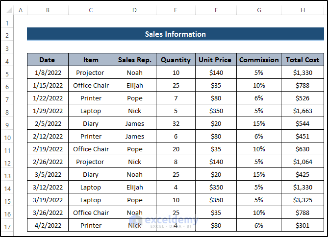
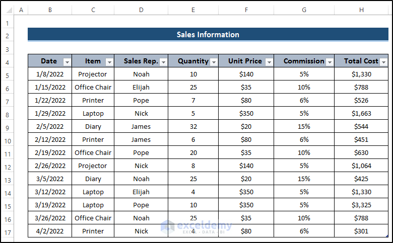
How to Combine Two Tables Using Power Query in Excel

To show the process, we have two datasets. One denotes the sales information, and the other is the region of sellers. In the sales information dataset, we set order date, item, sales rep., quantity, unit price, commission, and total cost.

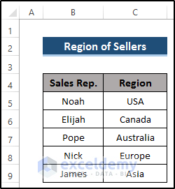
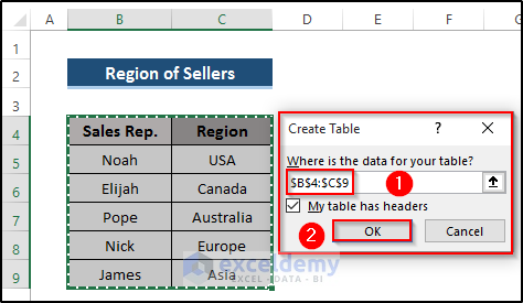
The region of sellers includes the sales rep. and their sales region. We would like to combine these two tables in Power Query.

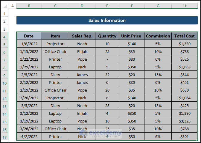
Step 1 – Converting the Datasets into Excel Tables

In the first dataset, select the range of cells B4 to H17.

Go to the Insert tab on the ribbon.
Select Table from the Tables group.

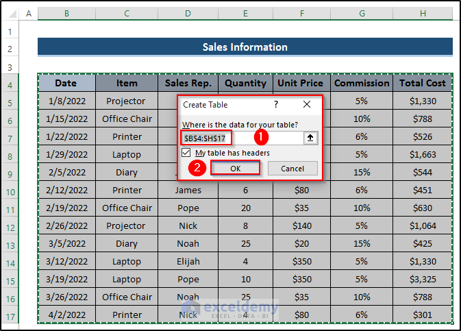
The Create Table dialog box.
As you selected the range of cells previously, it appears there automatically.
Check on My table has headers.
Click on OK.

Here’s the table.

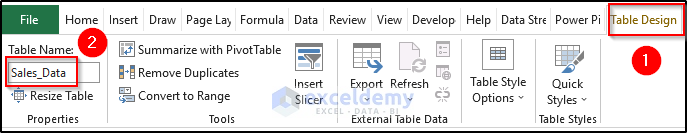
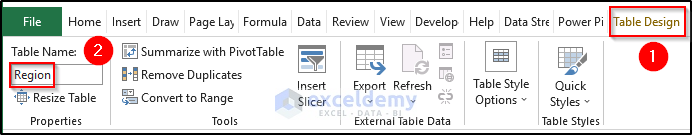
Select any cell on the table, and it will open the Table Design tab on the ribbon.
Select the Table Design tab on the ribbon and set the Table Name as Sales_Data from the Properties group.

In the second dataset, select the range of cells B4 to C9.

Go to the Insert tab on the ribbon.
Select Table from the Tables group.

The Create Table dialog box.
As you selected the range of cells previously, it appears there automatically.
Check on My table has headers.
Click on OK.

You will get the following result. See the screenshot.

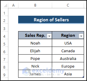
Select any cell on the table, and it will open up the Table Design tab on the ribbon.
Select the Table Design tab on the ribbon and set the Table Name as Region from the Properties group.

Read More: How to Perform Outer Join in Excel

Step 2 – Using Excel Power Query to Create a Connection Between the Two Tables

Select any cell on the first table.
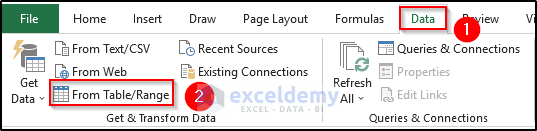
Go to the Data tab on the ribbon.
Select From Table/Range option from the Get & Transform Data group.

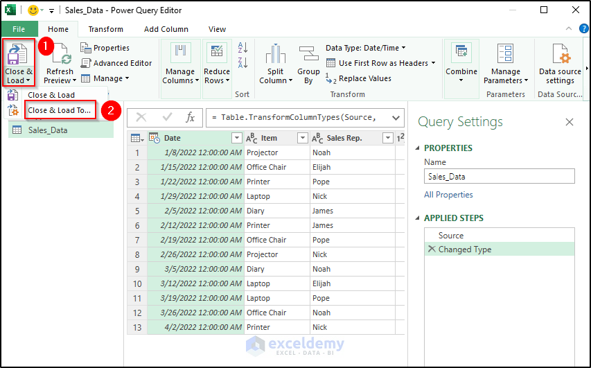
This will take the Sales_Data table into Power Query.
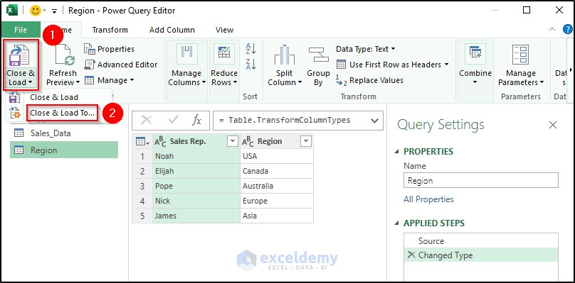
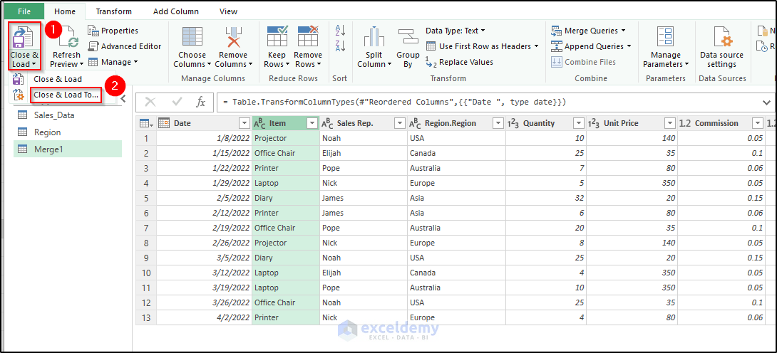
Select the Home tab on the ribbon.
Select the Close & Load drop-down option from the Close group.
Select the Close & Load To option from the Close & Load drop-down option.

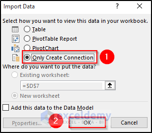
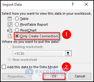
The Import Data dialog box will appear.
Select Only Create Connection from the Select how you want to view this data in your workbook section.
Click on OK.

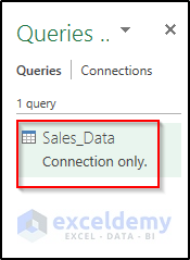
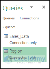
This will create a connection with the name of the table and appear in the Queries.
The Queries will appear on the right side of your workbook.

Select any cell on the second table.
Go to the Data tab on the ribbon.
Select From Table/Range option from the Get & Transform Data group.

This will take the Region table into Power Query.
Select the Home tab on the ribbon.
Select the Close & Load drop-down option from the Close option.
Select the Close & Load To option from the Close & Load drop-down option.

The Import Data dialog box will appear.
Select Only Create Connection from the Select how you want to view this data in your workbook section.
Click on OK.

This will create a connection with the name of the table and appear in the Queries.
The Queries will appear on the right side of your workbook.

Step 3 – Combining Two Tables into One in Power Query

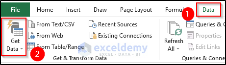
Select the Data tab on the ribbon.
Select Get Data drop-down option from the Get & Transform Data group.

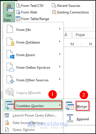
From the Combine Queries option, select Merge.

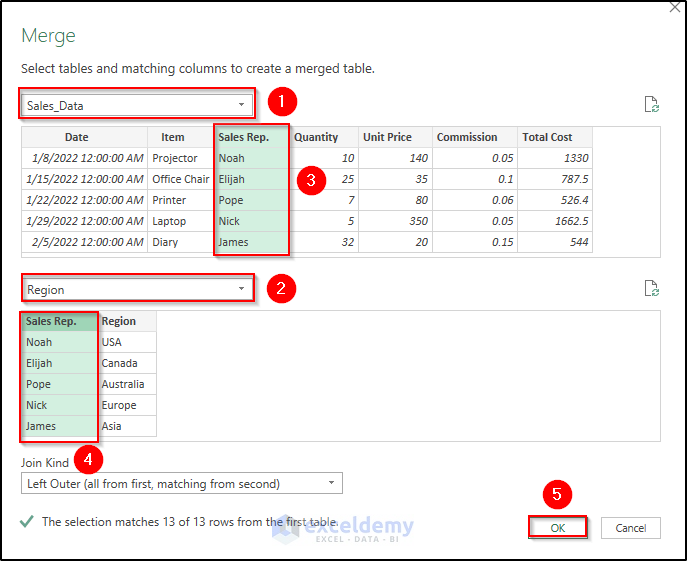
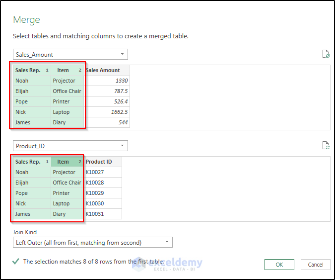
The Merge dialog box will appear.
From the drop-down option, select the Sales_Data table and then select the Region table from the second drop-down option.
Select the Sales Rep. Column for both tables to create a connection.
Click on OK.

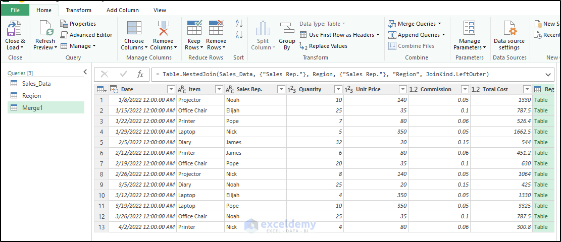
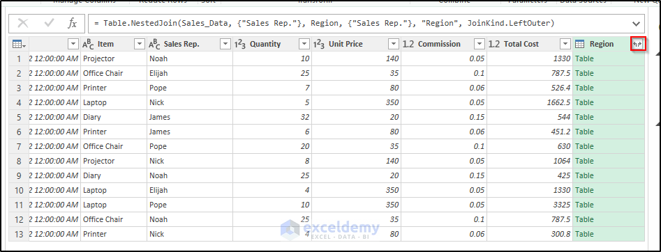
This will take you to Power Query. See the screenshot.

Step 4 – Importing the Combined Table into Excel

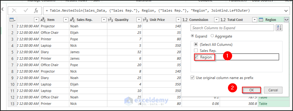
Select the two-sided arrow in the header.

You get a filter option. Select the Region option.
Click on OK.

You will get the region in this column. See the screenshot.

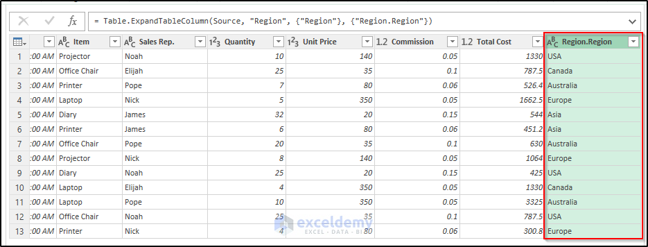
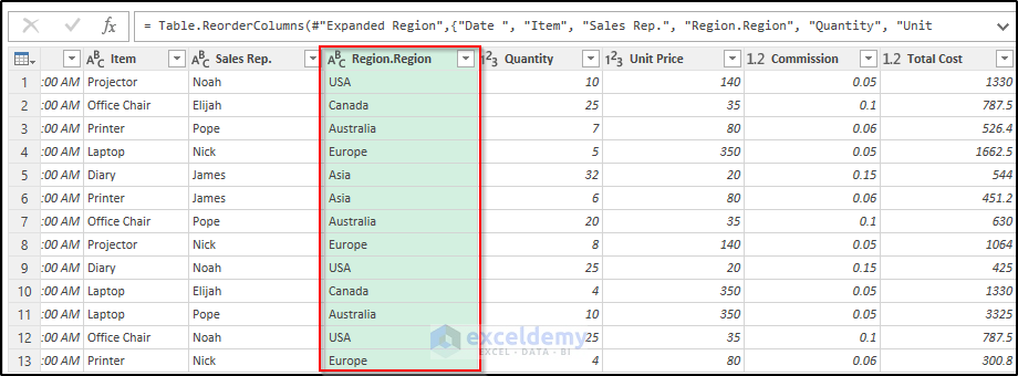
You can drag the region beside the sales rep.
Hold the header by clicking and set it in the desired place.

Select the Home tab on the ribbon.
Select the Close & Load drop-down option from the Close option.
Select the Close & Load To option from the Close & Load drop-down option.

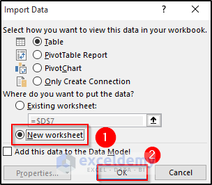
The Import Data dialog box will appear.
Select Table from the Select how you want to view this data in your workbook section.
Select the New Worksheet option to put the data.
Click on OK.

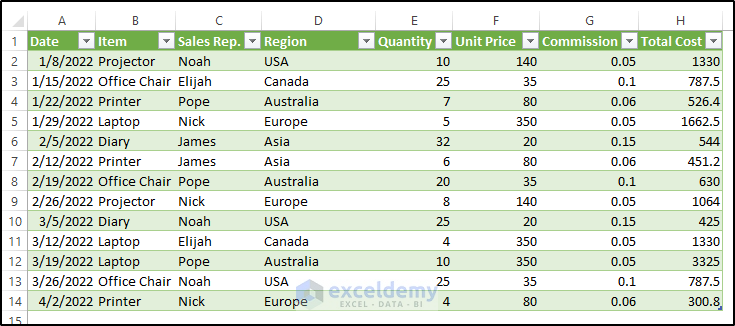
We will get the following result. See the screenshot.

How to Join Tables Based on Multiple Columns Using Power Query in Excel

Follow the procedure that we did previously to make connections between two tables.
Go to the Data tab on the ribbon.
Select Get Data drop-down option from the Get & Transform Data group.
From the Combine Queries option, select Merge.
In the Merge dialog box, press Ctrl and click the important columns one after another.
Continue with the merge.

How to Refresh the Combined Table in Excel

You can do the refresh from the Queries section which appears on the right side of the workbook.

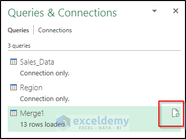
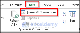
If the Queries pane disappears from your workbook, you can easily get it. To get this, you need to go to the Data tab on the ribbon. From the Queries & Connections group, select Queries & Connections.

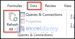
You can refresh the merged table from the Data tab where you must select Refresh All from the Queries & Connections group.

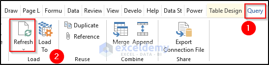
Otherwise, you need to click any cell on the merged table, it will open up the Query option on the ribbon. Then, select Refresh from the Load group.