How to Create a Full Outer Join in Excel – 2 Examples

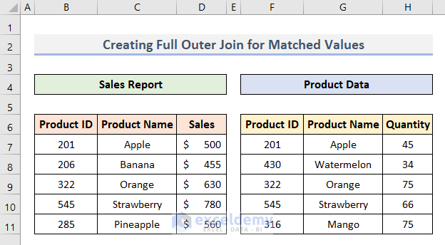
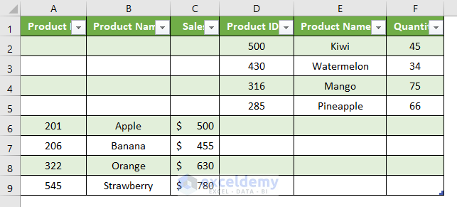
Example 1 – Create a Full Outer Join for Matched Values in Excel

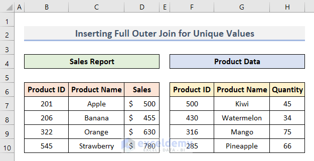
There are 2 sample tables. They showcase a Sales Report and Product Data.

To create a new table with all data:

• Click any cell in the first dataset.
• Go to the Data tab and select From Table/Range.

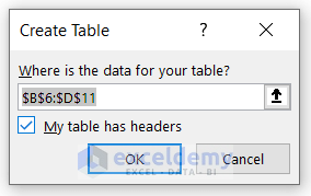
• In the Create Table window, the cell range to create a table is automatically selected.
• Click OK and the Power Query Editor will be displayed.

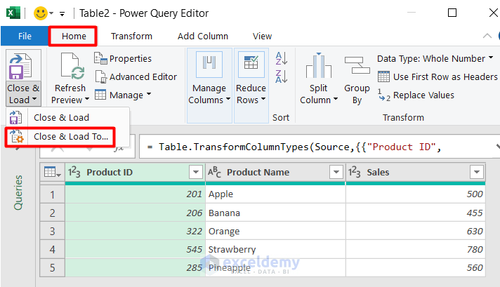
• Select Close & Load To in the Home tab.

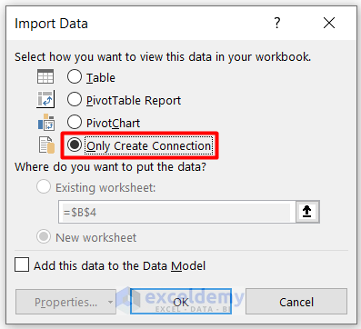
• Select Only Create Connection in the Import Data dialog box and click OK.

• Follow the same procedure for the Product Data table.
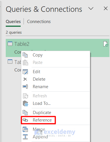
• You will see 2 connected tables in the Queries & Connections panel.

• Right-click Table2 and choose Reference.

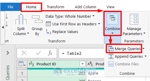
• Select Home > Combine > Merge Queries in the Power Query Editor window.

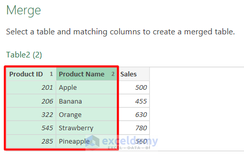
• In the Merge window, select Product ID and Product Name columns by pressing Ctrl.

• Choose Table3 and select the columns that are in Table2.

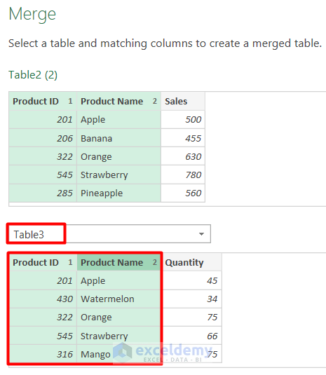
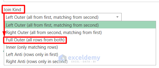
• Choose Full Outer (all rows from both) as Join Kind.

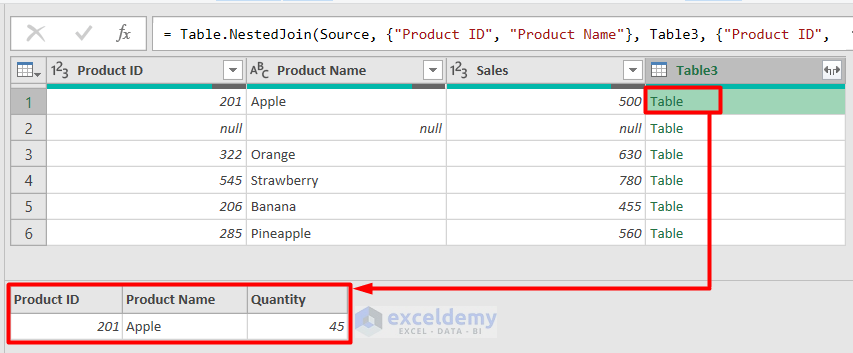
A new column is added: you can see the row values by left-clicking.

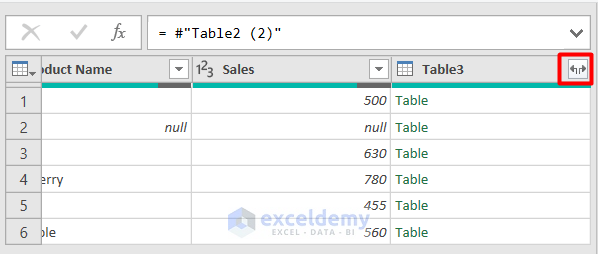
• Expand this column by pressing the both-sided arrow shown below.

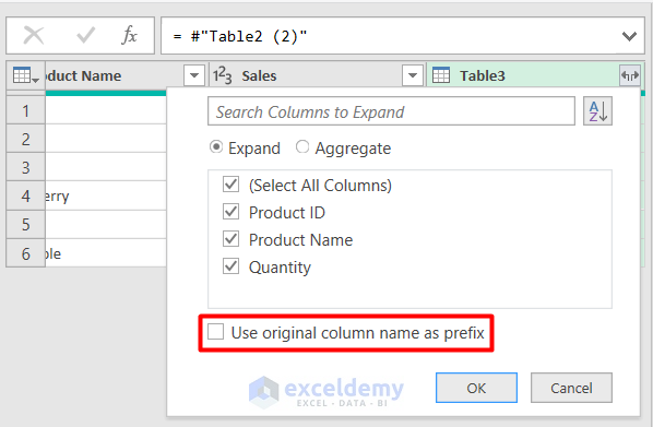
You will see the list of columns in Table3.

• Select the columns you need to show after merging. Here, all columns are selected. You can but deselect them by checking Use original column name as prefix.

• Click OK.
• In the Import Data window, select Table and New worksheet.

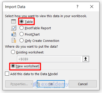
• Click OK and you will get a Full Outer Join table:

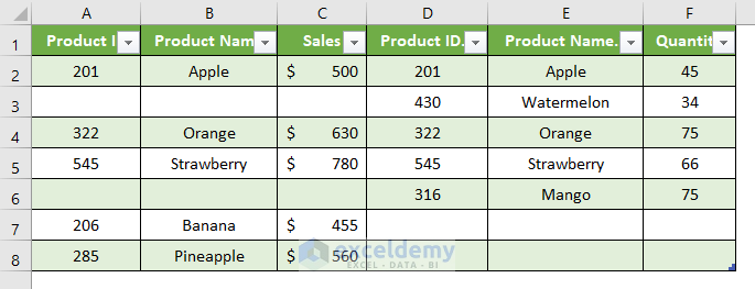
Matched values are aligned together and the rows with unique values have blank cells.

Read More: How to Perform Outer Join in Excel

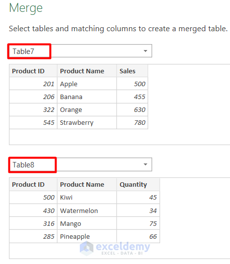
Example 2 – Perform a  Full Outer Join for Unique Values in Excel

These are the sample datasets containing unique values.

• Connect both tables using the Power Query Editor as described in the first example.
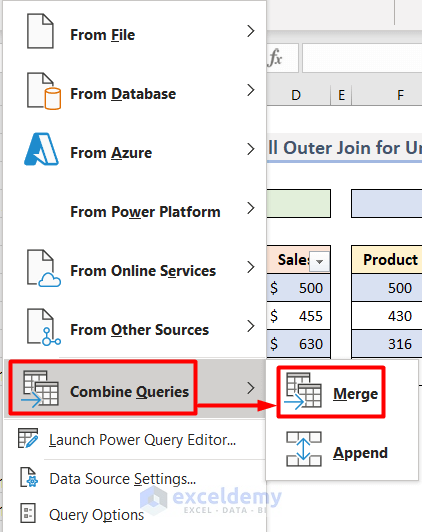
• Go to the Data tab and click Get Data.

• Choose Merge in Combine Queries.

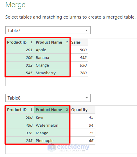
• In the Merge window, choose Table7 and Table8.

• Select Product ID and Product Name from each table.

• Select Full Outer (all rows from both) in Join Kind.

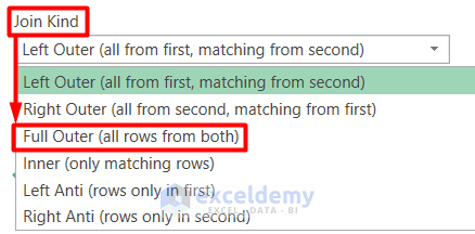
• Click OK.
• In the Power Query Editor, expand the last column with the selections shown below.
• Uncheck Use original column name as prefix.

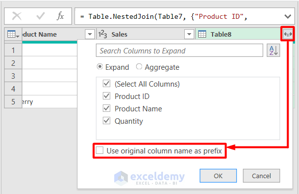
• Click OK and choose Table and New Worksheet in the Import Data dialog box.

• Click OK to see the output.

Read More: How to Inner Join in Excel

Download Practice Workbook

Download the practice file.

Related Articles

• How to Combine Two Tables Using Power Query in Excel
• How to Perform Left Join in Excel
• How to Perform Left Outer Join in Excel
• How to Create Cross Join in Excel

<< Go Back to Power Query Excel | Learn Excel