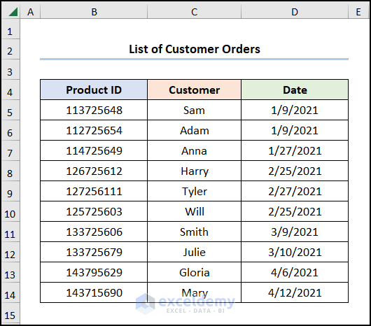
Consider the List of Customer Orders containing the “Product ID”, “Customer”, and “Date”.
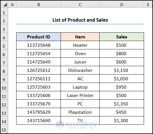
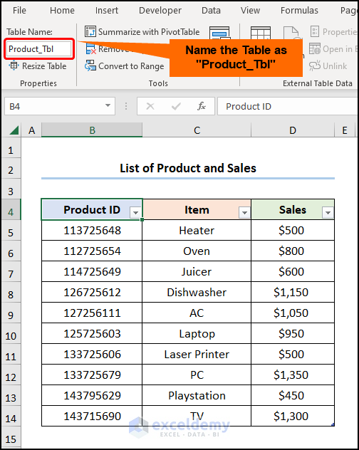
Mind this List of Products and Sales with “Product ID”, “Item”, and “Sales” in USD.
Perform an outer join based on the common “Product ID”:
Method 1 – Using the IFERROR and the VLOOKUP Functions
Steps:
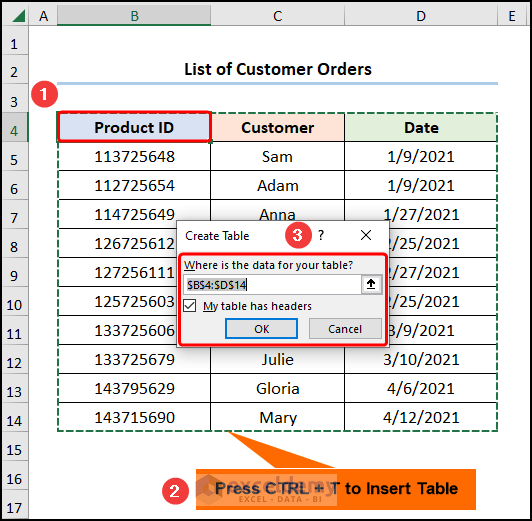
- Go to B4 >> press CTRL + T to create and insert a Table.
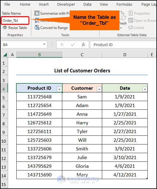
- Name the Table “Order_Tbl”.
- Create a second Table and name it “Product_Tbl”.
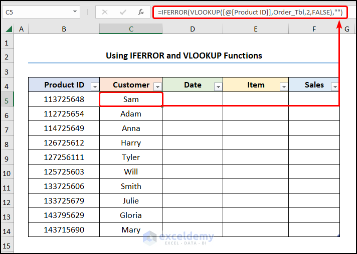
- Go to C5 and enter the formula below.
=IFERROR(VLOOKUP([@[Product ID]],Order_Tbl,2,FALSE),"")
Product ID refers to the column header, whereas Order_Tbl is the Table range.
Formula Breakdown:
- VLOOKUP([@[Product ID]],Order_Tbl,2,FALSE) → looks for a value in the left-most column of a table, and returns a value in the same row from a specified column. Here, [@[Product ID]] ( lookup_value argument) is mapped in the Order_Tbl (table_array argument) array in the “Order” worksheet. 2 (col_index_num argument) represents the column number of the lookup value. FALSE (range_lookup argument) refers to the Exact match of the lookup value.
- Output → “Sam”
- IFERROR(VLOOKUP([@[Product ID]],Order_Tbl,2,FALSE),””) → becomes
- IFERROR(“Sam”,“”) → returns value_if_error if the expression has an error. Otherwise, the value of the expression. Here, “Sam” is the value argument, and “”(Blank) is the value_if_error argument. The function returns “Sam”.
- Output → “Sam”
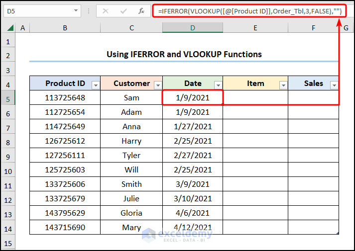
- Go to the D5 and use the expression below.
=IFERROR(VLOOKUP([@[Product ID]],Order_Tbl,3,FALSE),"")
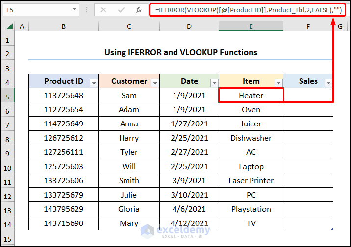
- Enter the equation below in E5.
=IFERROR(VLOOKUP([@[Product ID]],Product_Tbl,2,FALSE),"")
The Product_Tbl represents the Table range.
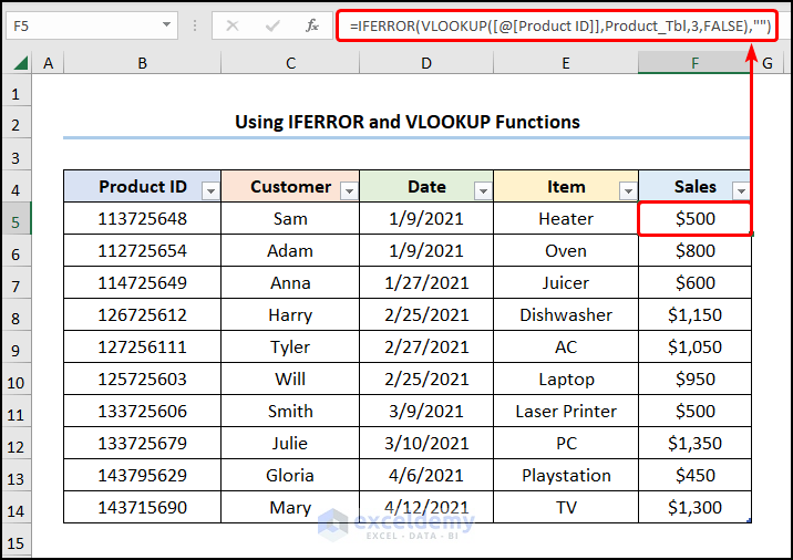
- Select F5 and enter the expression in the Formula Bar.
=IFERROR(VLOOKUP([@[Product ID]],Product_Tbl,3,FALSE),"")
This is the output.
Method 2 – Utilizing the Power Query Editor
Steps:
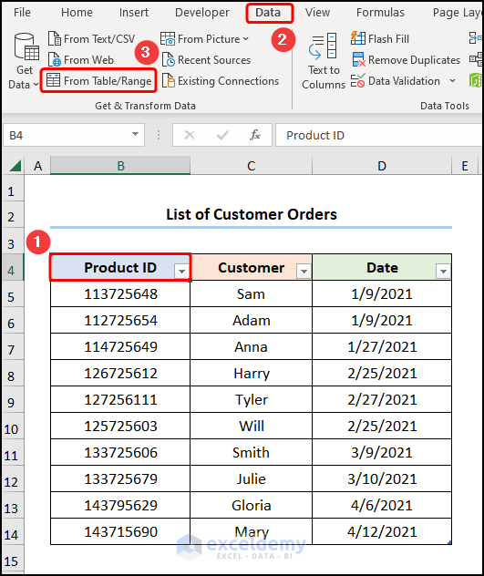
- Select B4 in the “Order” worksheet >>go to the Data tab >> select From Table/Range.
- Check Only Create Connection >> click OK.
Repeat the procedure for the Table in the “Order” worksheet.
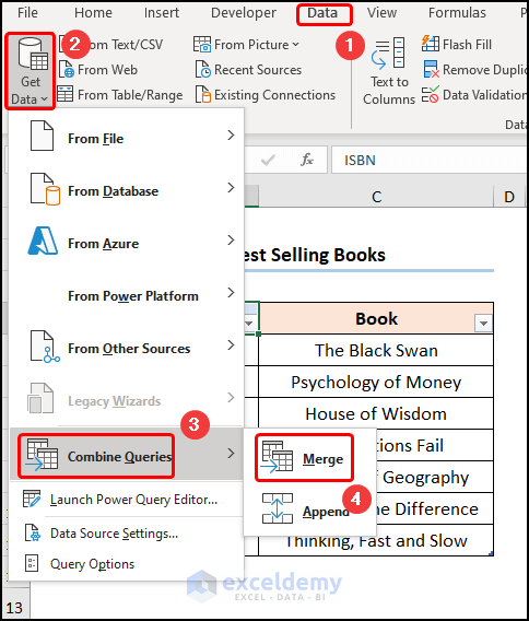
- Go to Get Data >> select Combine Queries >> choose Merge.
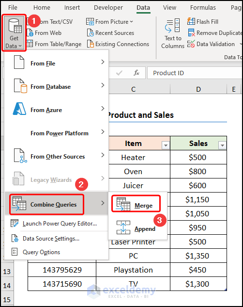
- Follow the steps shown in the GIF below.
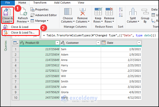
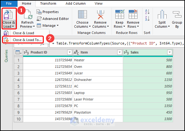
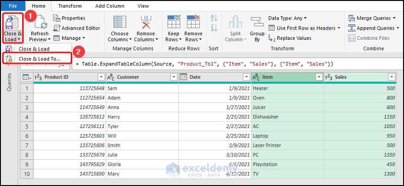
- Click Close & Load To.
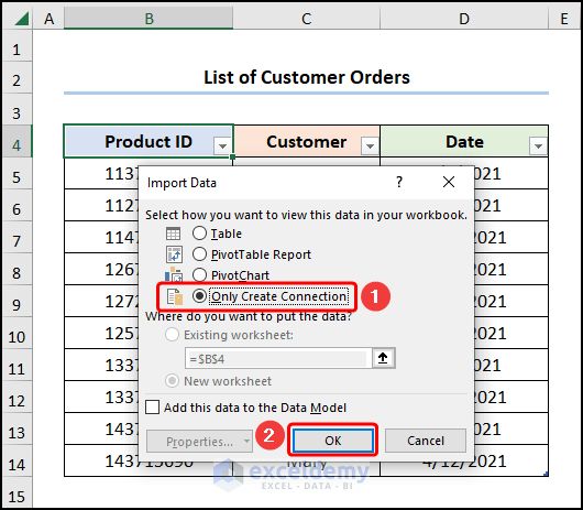
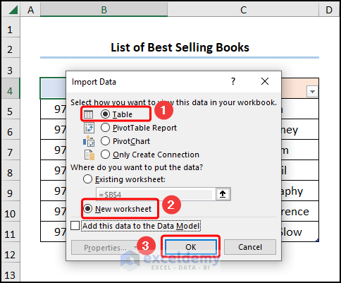
- In the Import Data window, check Table and New Worksheet >> click OK.
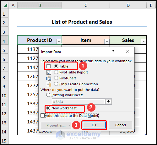
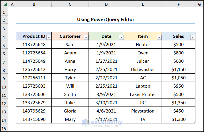
This is the final output.
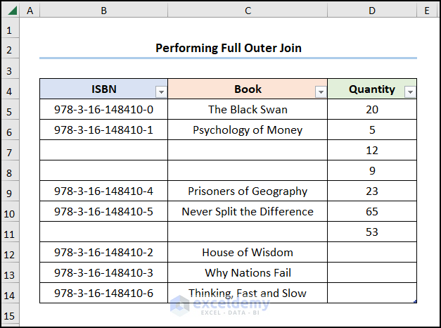
How to Execute a Full Outer Join in Excel
Perform a full outer join combining all rows in the two datasets/tables into one.
Steps:
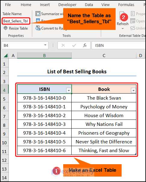
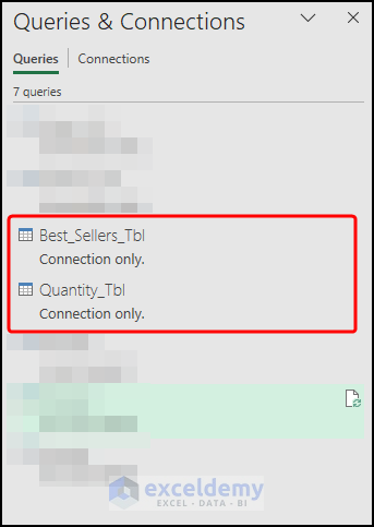
- Go to the “Best Sellers” worksheet >> create a Table and name it “Best_Sellers_Tbl”.
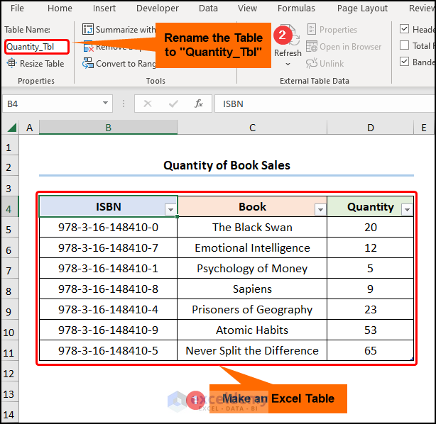
- Repeat the previous step in the “Quantity” worksheet to create the “Quantity_Tbl”.
- Load and Establish a Connection between Tables by following the steps described above.
- Go to Get Data >> choose Merge in Combine Queries.
- Follow the steps shown in the GIF below.
- Load the data into a New Worksheet as a Table.
This is the output.
Read More: How to Perform Left Join in Excel
How to perform an Inner Outer Join in Excel
Steps:
- Load the Tables into the PowerQuery editor >> Merge the two queries as shown below.
- Close & Load the transformed data into a new worksheet.
Read More: How to Inner Join in Excel
Practice Section
Practice here.
Download Practice Workbook
Related Articles
- How to Combine Two Tables Using Power Query in Excel
- How to Perform Left Outer Join in Excel
- How to Create Cross Join in Excel
<< Go Back to Power Query Excel | Learn Excel
Get FREE Advanced Excel Exercises with Solutions!
