This tutorial will demonstrate how to perform left outer join to merge data tables in Excel.
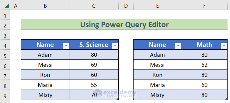
We’ll use the sample dataset below, which contains two tables. In the first table we have Social Science marks for some students, while in the second table we have Math marks for the same students. Create a table simply by selecting your data range and pressing Ctrl+T.
Method 1 – Merging Tables Using Power Query Editor
Power Query, also known as “Get & Transform Data”, is a powerful tool available in Microsoft Excel 2010 and later versions, that can clean up and automate data.
Steps:
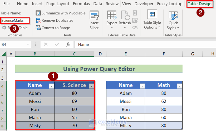
- Select the first table.
- Go to the Table Design tab >> Table Name.
- Set the Table Name (in this case, ScienceMarks).
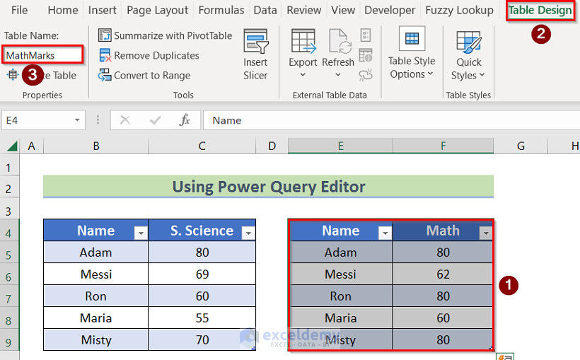
- Repeat the process to name the second table as MathMarks.
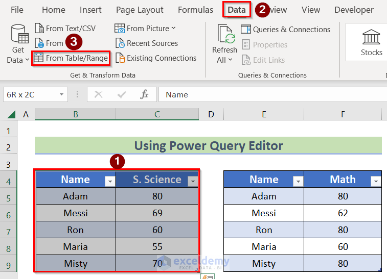
- Select the data table.
- Go to the Data tab >> From Table/Range.
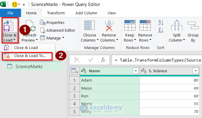
The Power Query Editor opens, displaying the specified data.
- Click Close & Load to create the connection.
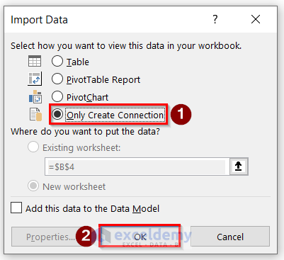
- In the Import Data tab, select the Only Create Connection option.
- Click OK.
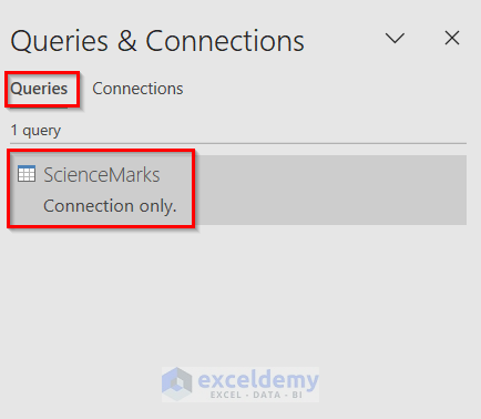
In the Queries and Connection tab, the new connection is displayed.
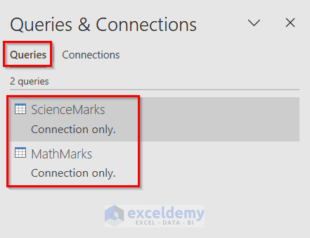
- Repeat the whole process for the second table.
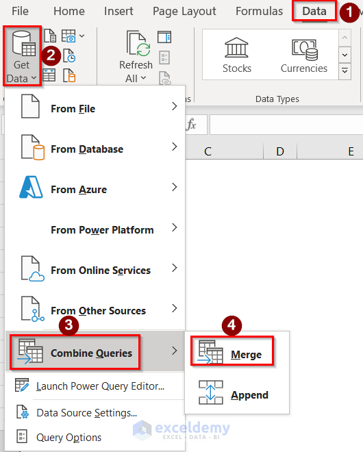
- Go to the Data tab >> Get Data >> Combine Queries >> Merge.
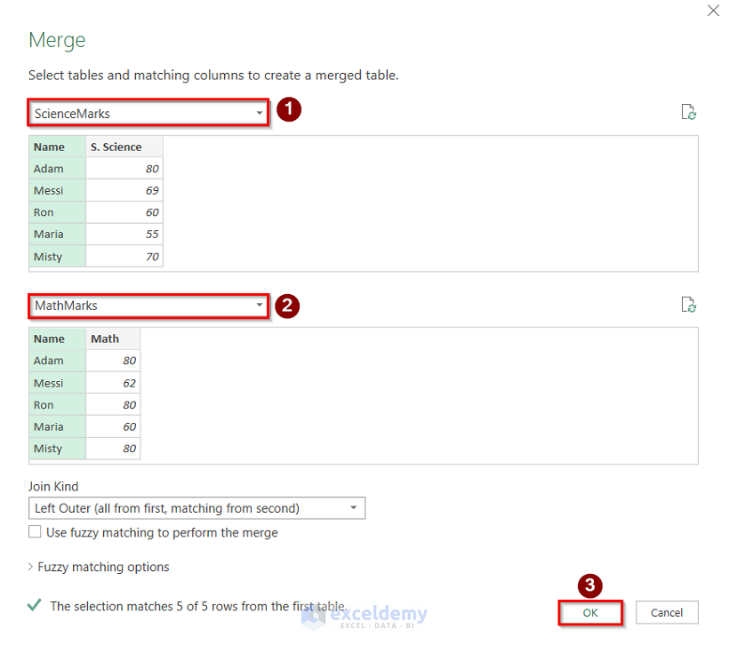
The Merge window opens.
- Select the tables accordingly.
- Select the first columns of the tables.
- Click OK.
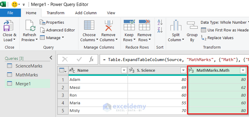
In the Power Query window, the table where both tables have been merged is displayed.
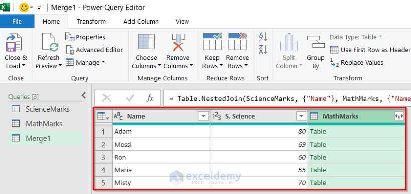
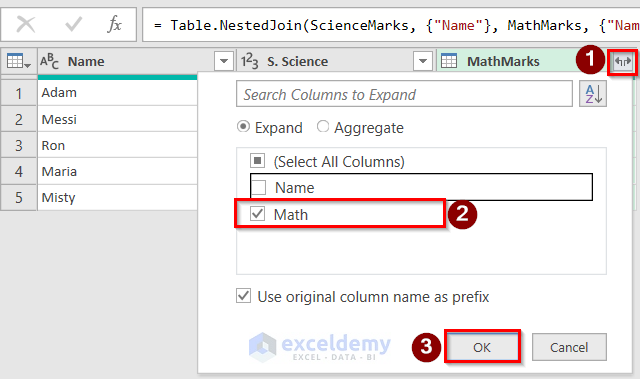
- Click on the arrow sign of the new column.
- Select the data you want to show there (in this case, select the Math option).
- Click OK.
The data in the third column is displayed.
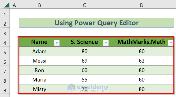
- Click Close and Load to return the final result.
Read More: How to Combine Two Tables Using Power Query in Excel
Method 2 – Using VLOOKUP Function
The VLOOKUP function function is generally used to extract data based on a lookup value in a column or a range of cells.
Steps:
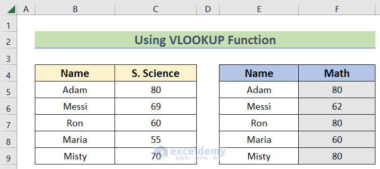
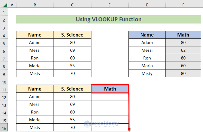
- Create a data table similar to the image below.
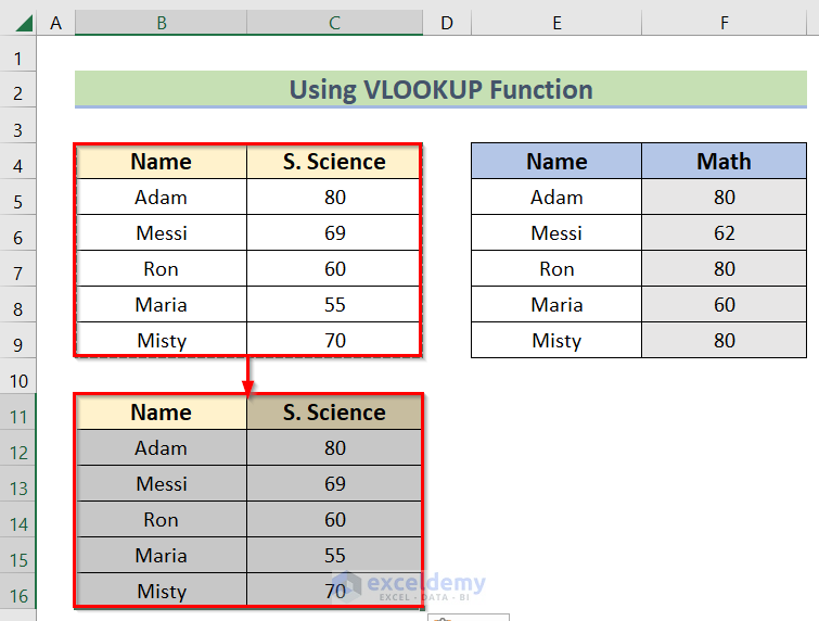
- Select the first table and press the Ctrl + C option to copy it.
- Press Ctrl + V to paste the value in another blank cell.
- Enter the following formula in cell D11:
=VLOOKUP(B11,$E$4:$F$9,2,FALSE)
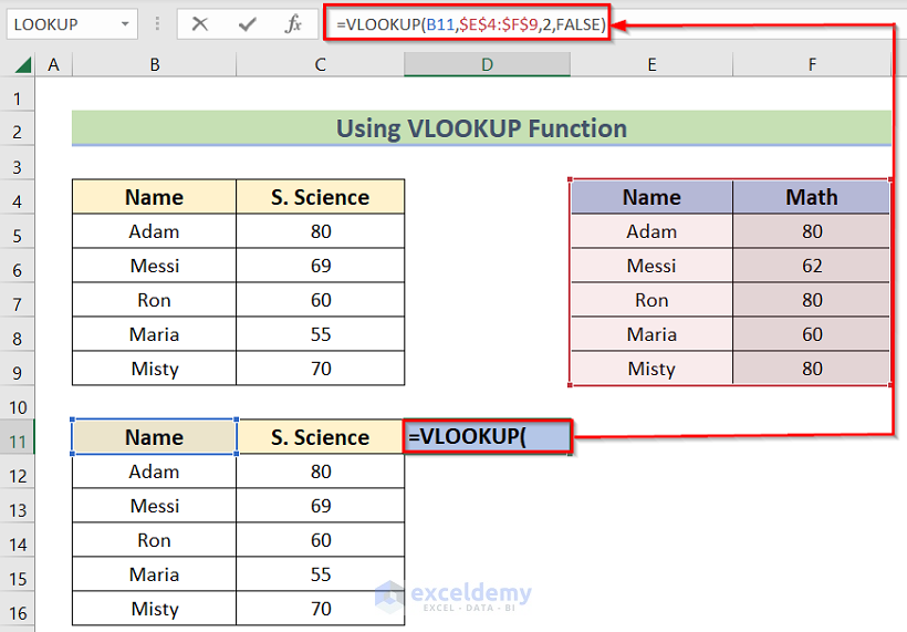
In the formula, the first value (B11) is the look-up value, the second portion $E$4:$F$9 portion is the table array we will use, and the last portion (2) represents the second column of the selected data range (the range from which to return corresponding values).
The result for this cell is returned, in this case the 2nd column of the E4:F9 range data, Math.
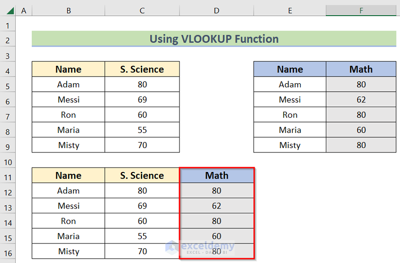
- Use the Fill Handle to copy the formula to all the cells of this column.
The data from the second column is returned, namely the merging of the two data tables. In this new table, the first two columns are the values of the first table, and in the third column are the values of the second table.
Read More: How to Perform Left Join in Excel
Download Practice Workbook
Related Articles
- How to Inner Join in Excel
- How to Perform Outer Join in Excel
- How to Create Full Outer Join in Excel
- How to Create Cross Join in Excel
<< Go Back to Power Query Excel | Learn Excel
Get FREE Advanced Excel Exercises with Solutions!
