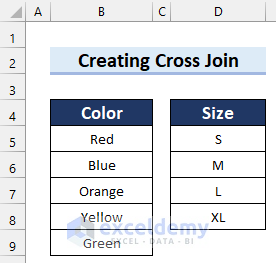
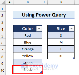
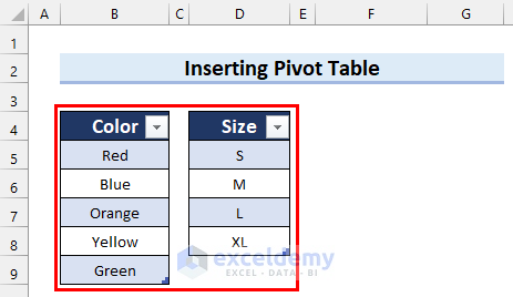
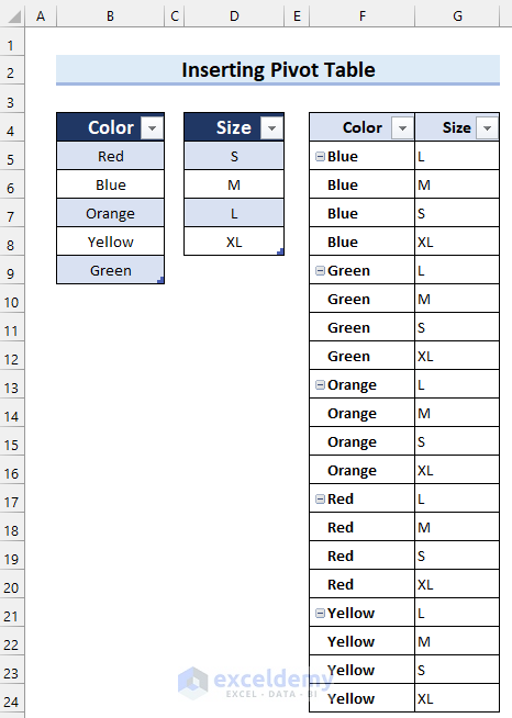
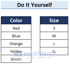
How to Create Cross Join in Excel (3 Simple Ways)

The sample dataset contains the Color and Sizes of a t-shirt. We will Cross Join these tables to get all the available variations of that t-shirt.

Dataset for How to Create Cross Join in Excel

Method 1 – Use Power Query to Create a Cross Join in Excel7

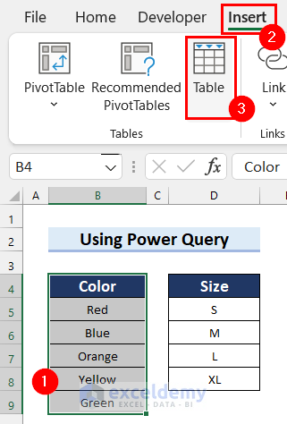
Step 1 – Create a Table

Select the data range.
Go to the Insert tab.
Select Table.

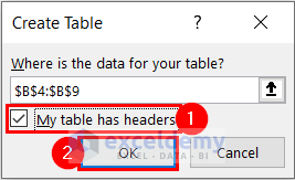
Inserting Table to Create Cross Join in Excel

The Create Table dialog box will appear.
Check the My table has headers option.
Select OK.

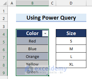
Using Create Table Dialog Box for Creating Table

You will get a table.

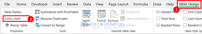
Getting Table with Selected Data Range in Excel

Go to the Table Design tab.
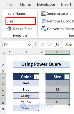
Write the Table Name.

Setting Table Name from Table Design Tab in Excel

Create a table for the other data range and name it.

Creating and Naming Table from Another Data Range in Excel

Step 2 – Import the Tables and Load as Connections

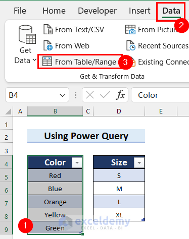
Select a table.
Go to the Data tab.
Select From Table/Range.

Using From Table/Range Command to Import Table Using Data Tab

The table is imported to Power Query.
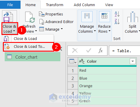
Select the drop-down option for Close & Load.
Select Close & Load to.

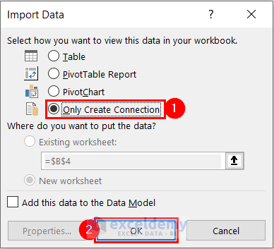
Selecting Close & Load for Making Cross Join in Excel

The Import Data dialog box will appear.
Select Only Create Connection.
Select OK.

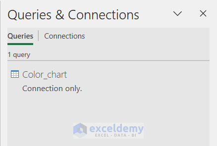
Using Import Data Dialog Box to Only Create Connections for Cross Join in Excel

You will see that the Queries & Connections task pane appears on the right side of the screen.
1 Query is added as Connection only.

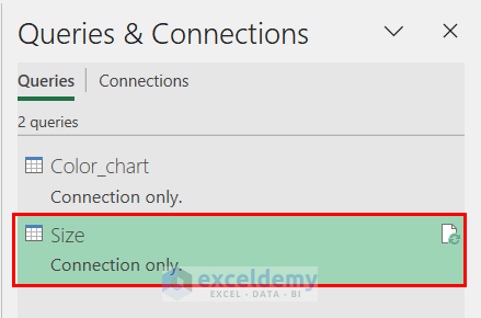
Adding Color_chart as Connection Only Query

Add the other table as a Connection only query in the same way.

Adding Size as Connection Only Query

Step 3 – Create a Reference Query and a Custom Column

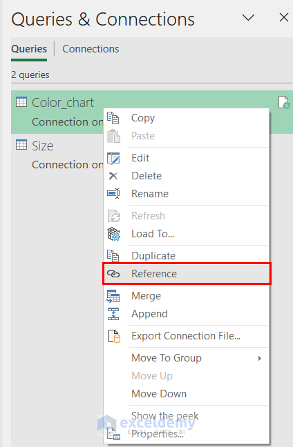
Right-click on the query that you want as your first column in the cross-join.
Select Reference.

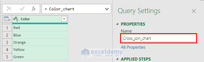
Selecting Reference to Create Reference Query in Excel

Change the name of the query.

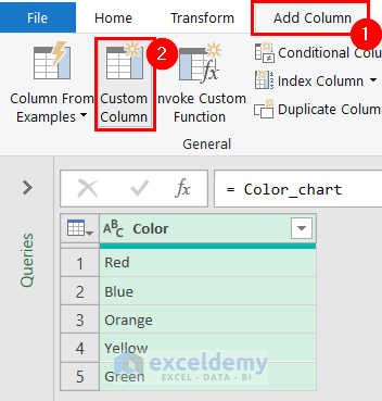
Changing Name of Query to Cross Join in Excel

Go to the Add Column tab.
Select Custom Column.

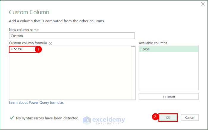
Adding Column to Cross Join in Excel

The Custom Column dialog box will appear.
In the Custom column formula section, write the name of the other table with which you want to create a cross-join.
Select OK.

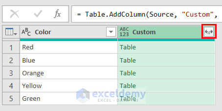
Custom Column Dialog Box for Creating Cross Join in Excel

You’ll get a new custom column in the table.
Select the Expand button.

Adding a New Custom Column And Expanding It for Cross Join

A drop-down menu will appear.
Select the column you want from the table.

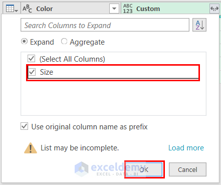
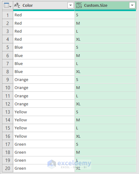
Selecting Preferred Column for Cross Join in Excel

We got the Cross Join.

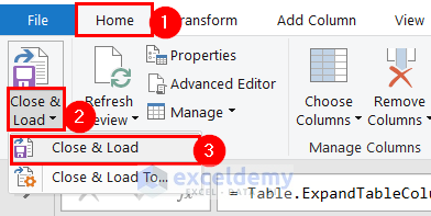
Cross Join Chart in Excel Power Query

Step 4 – Load as Table

Go to the Home tab.
Click on the drop-down option for Close & Load.
Select Close & Load.

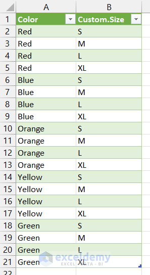
Selecting Close & Load to Load the Cross Join Chart

You will see that the Cross Join is loaded in a table in a new Excel sheet.

Final Cross Join Table That is Loaded in Excel Sheet

Step 5 – Add New Data

Add new data to the table.

Add New Data in Excel Table

Select the Refresh button in the Cross Join from Queries & Connections.

Refresh to Add New Data in It

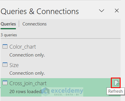
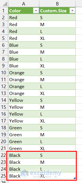
The new data will be added to the Cross Join table.

New Data Are Loaded in Cross Join Table

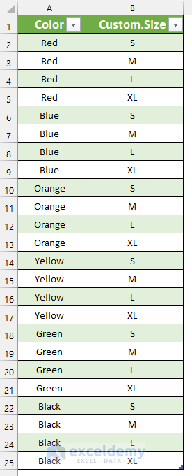
Final Output:

Here’s the final Cross Join table after formatting.

Final Cross Join Table After Formatting in Excel

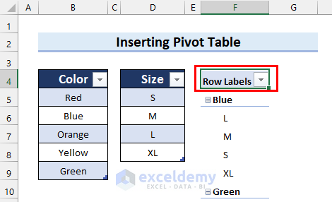
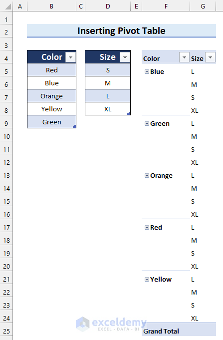
Method 2 – Insert a Pivot Table to Create a Cross Join in Excel

Steps:

Insert tables and name them by following the Step 1 of Method 1.

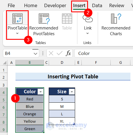
Creating Tables with The Data Ranges And Use Them for Cross Join in Excel

Select the table which you want as your first column.
Go to the Insert tab.
Select PivotTable.

Inserting Pivot Table in Excel

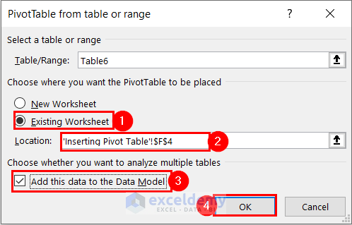
The PivotTable from table or range dialog box will appear.
Select Existing Worksheet.
Select the Location where you want the table.
Check the Add this data to the Data Model option.
Select OK.

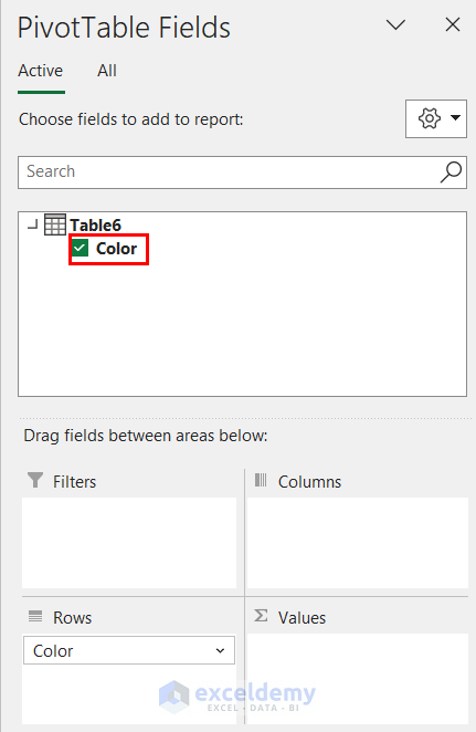
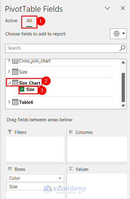
Using PivotTable from table or range Dialog Box in Excel

The PivotTable Fields task pane will appear on the right side of the screen.
Select the column from the table, and it will be added to the Rows area.

Adding Column to The Rows Area to Create Cross Join in Excel

Select the All tab.
Select the table that you want as the second column of your Cross Join.
Check the column name to add it to the Rows area. We have only one column in the table.

Adding Second Column to The Rows Area of Pivot Table

You will get the Pivot Table.
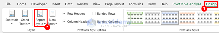
Select any cell of the Pivot Table.

Selection Any Cell of The Pivot Table to Change Table Design

Go to the Design tab.
Select Report Layout.

Selecting Report Layout from Design Tab

A drop-down menu will appear.
Select Show in Tabular Form.

Choosing Show in Tabular Form

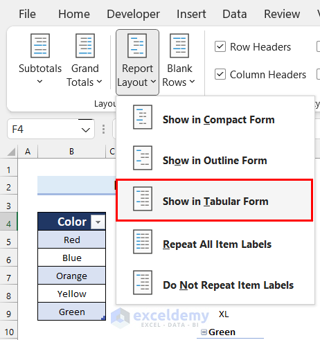
We got the Pivot Table in tabular form.

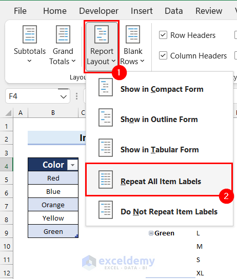
Pivot Table in Tabular Form to Get Cross Join in Excel

Select Report Layout again.
Select Repeat All Item Labels.

Selecting Repeat All Item Labels

Select Grand Totals.
Select Off for Rows and Columns.

Removing Grand Totals in Excel

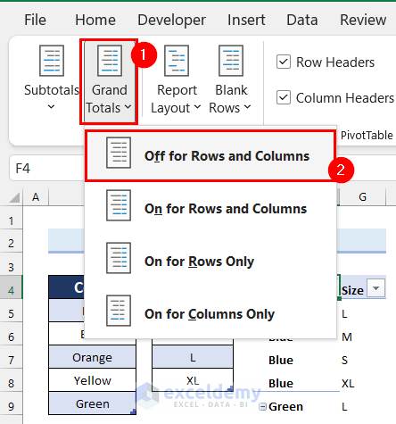
This completes the Cross Join.

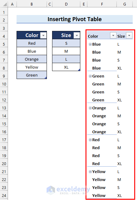
Getting Cross Join in Form of Pivot Table in Excel

We have added a border to the Pivot Table.

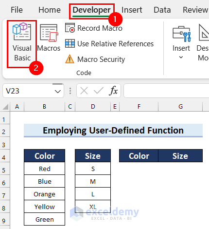
Final Cross Join Pivot Table in Excel

Method 3 – Use a User-Defined Function to Create a Cross Join in Excel

Steps:

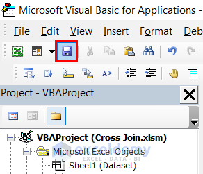
Go to the Developer tab.
Select Visual Basic.

Opening Visual Basic Editor to Create User-Defined Function in Excel

The Visual Basic editor window will open.
Select the Insert tab.
Select Module.

Opening a Module to Write VBA Code

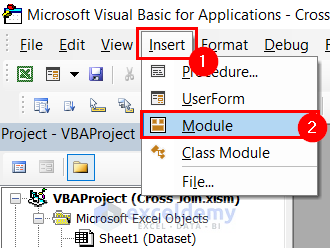
A Module will open.
Insert the following code in that Module.

Function cross_join(rng1 As Range, rng2 As Range) As Variant
            Dim total_count As Integer
            Dim output_arr As Variant
            Dim row_offset As Integer
            total_count = rng1.Rows.Count * rng2.Rows.Count
            ReDim output_arr(0 To total_count - 1, 0 To 1)
            row_offset = 0
            For p = 1 To rng1.Rows.Count
            For q = 1 To rng2.Rows.Count
            output_arr(row_offset, 0) = rng1.Cells(p, 1).Value2
            output_arr(row_offset, 1) = rng2.Cells(q, 1).Value2
            row_offset = row_offset + 1
            Next q
            Next p
            cross_join = output_arr
End Function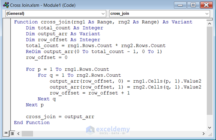

VBA Code for User-Defined Function for Cross Join in Excel

How Does the Code Work?

We created a Function named cross_join as a Variant.
We declared a variable named total_count as Integer, output_arr as Variant, and row_offset As Integer.
We used Rows.Count Property to get the total_count.
We used two For Next Loops to go through all the columns of both ranges and concatenate each value to create new ones.
We ended the Function.

Save the code and go back to your worksheet.

Saving VBA Code for Used-Defined Function

Select the cell where you want the Cross Join. We selected cell F5.
In cell F5, insert the following formula.

=cross_join(B5:B9,D5:D8)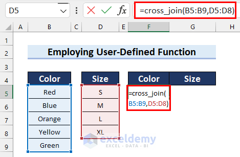

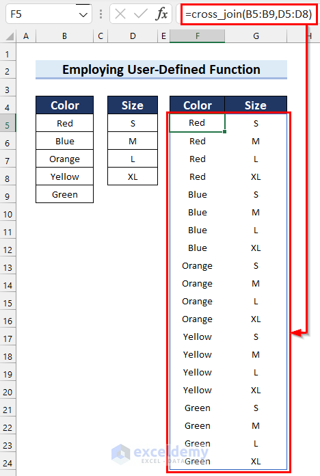
Using the User-Defined Function for Cross Join in Excel

Press Enter and you will get the Cross Join.

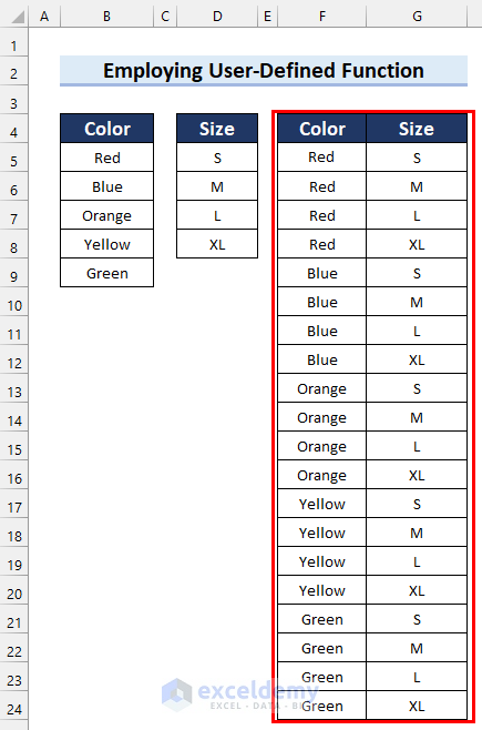
Getting Output from the cross_join Function

We have added a border.

Final Output of Cross Join From the User-Defined Function

Things to Remember

If you are working with VBA, you must save the Excel file as Excel Macro-Enabled Workbook.

Practice Section

We have provided a practice sheet for you to test these methods.

Practice Sheet for How to Create Cross Join in Excel

Download the Practice Workbook

Creating Cross Join.xlsm

<< Go Back to Power Query Excel | Learn Excel

Get FREE Advanced Excel Exercises with Solutions!

4 Comments

Rahul Feb 1, 2024 at 9:08 PM

Wonderfully Explained, was very helpful !!!!!
- Reply
  Shamima Sultana Feb 4, 2024 at 9:47 AM
  
  Hello Rahul,
  
  You are most welcome.
  
  Regards
  ExcelDemy
Robert Thompson Dec 17, 2024 at 10:58 PM

Or you can do it in a formula. It works better if you convert your original columns (Colors and Sizes) to Excel tables. But the below also works with Named Ranges or original ranges (e.g., B5:B9).

=LET(LenX, ROWS(Colors),
LenY, ROWS(Sizes),
Seq, SEQUENCE(LenX*LenY,,0),
Array1, XLOOKUP(INT((Seq)/LenY)+1, SEQUENCE(LenX), Letters, “”),
Array2, XLOOKUP(MOD(Seq,LenY), SEQUENCE(LenY,,0), Numbers, “”),
HSTACK(Array1, Array2))

This can then be used to define a Lambda function named “CrossJoin”:
=LAMBDA(Table1,Table2,
LET(LenX,ROWS(Table1),
LenY,ROWS(Table2),
Seq,SEQUENCE(LenX*LenY,,0),
Array1,XLOOKUP(INT((Seq)/LenY)+1,SEQUENCE(LenX),Table1,””),
Array2,XLOOKUP(MOD(Seq,LenY),SEQUENCE(LenY,,0),Table2,””),
HSTACK(Array1, Array2)))

Now you can simply call:
=CrossJoin(Colors, Sizes)
- Reply
  Shamima Sultana Dec 18, 2024 at 1:08 PM
  
  Hello Robert Thompson,
  
  Thank you for sharing this useful approach! The formula-based method is indeed a powerful alternative to Power Query and VBA.
  Using LET and LAMBDA makes it dynamic and reusable, especially with named ranges or tables. This approach is great for those who prefer formula-based solutions and want to avoid VBA or external tools.
  Your explanation is clear, and the CrossJoin LAMBDA function adds even more flexibility. It’s a fantastic addition to the methods mentioned in the article. Thanks for contributing this valuable insight!
  
  Regards
  ExcelDemy