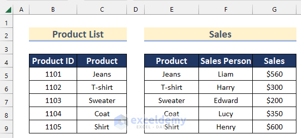
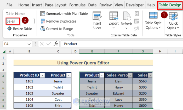
There are 2 datasets below. The first dataset contains Product ID and Name. The second one contains Product Name, salesperson’s name, and value of Sales.
Method 1 – Using the Power Query Editor to Perform Left Join in Excel
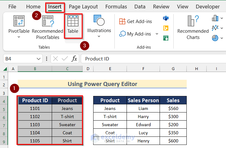
Step 1: Create Tables in Excel
- Select B4:C9.
- Go to the Insert tab >> click Table.
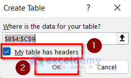
- In Create Table, the cell range is selected.
- Check My table has header option.
- Click OK.
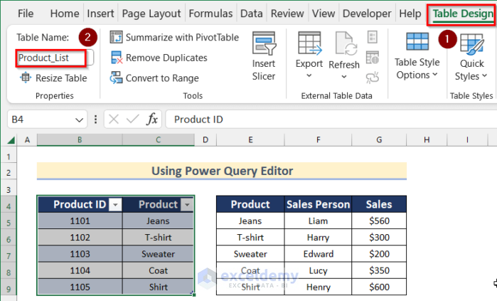
- Go Table Design >> name the table in Table Name. Here, Product_List.
- Create a table for E4:G9.
- In Table Design >>Name it Sales in Table Name.
Step 2: Create Connections in Power Query Editor
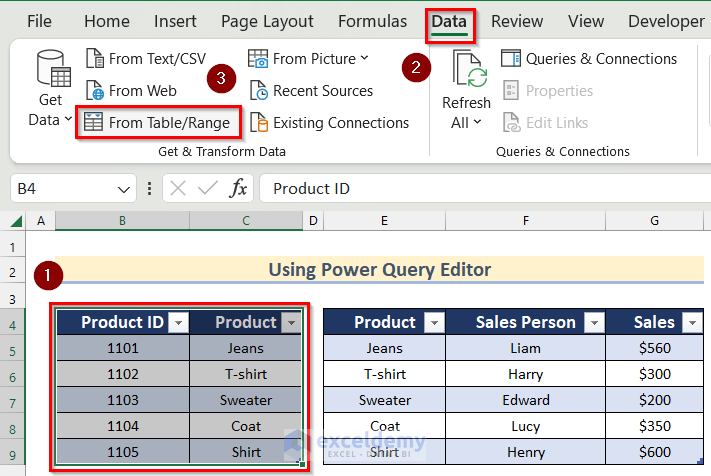
- Select the Product_List table.
- Go to the Data tab >> click From Table/Range.
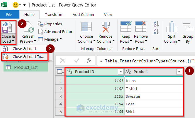
- The table will open in the Power Query Editor.
- Click Close & Load >> select Close & Load To.
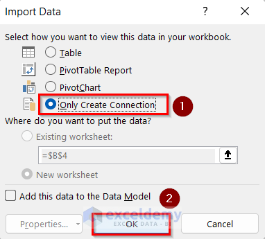
- In Import Data, select Only Create Connection.
- Click OK.
- Create a connection for the Sales Table.
Step 3: Merge Tables
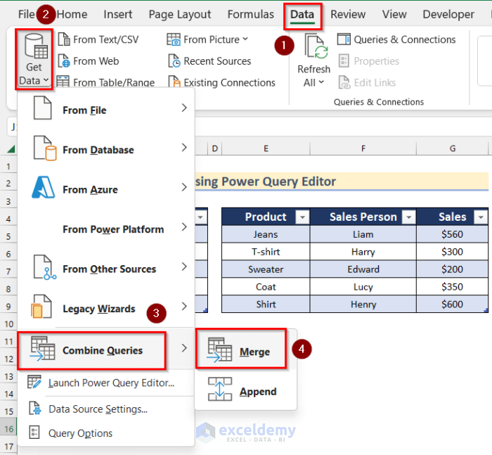
- Go to the Data tab >> click Get Data >> click Combine Queries >> select Merge.
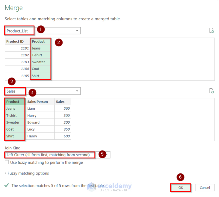
- In Merge, select the Product_List table and its Product column.
- Select the Sales table and its Product column.
- Select Left Outer as Join Kind.
- Click OK.
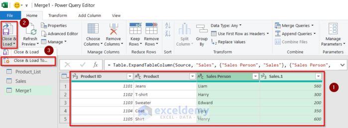
- Merge1 table will open in the Power Query Editor.
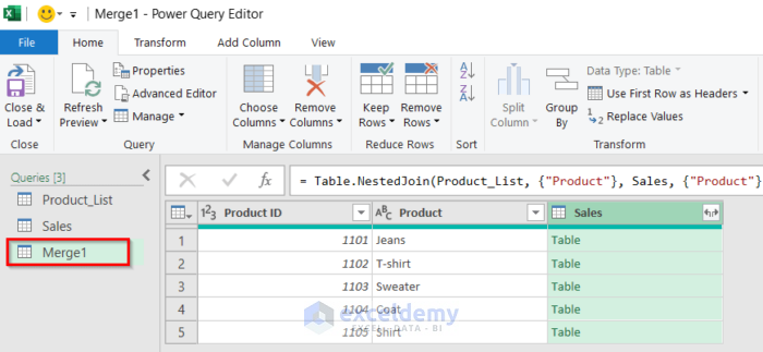
- Click the sign shown in the image below.
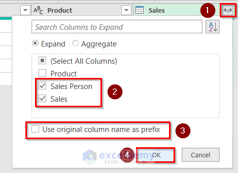
- Check Sales Person and Sales.
- Uncheck Use original column name as prefix.
- Click OK.
The two columns are merged.
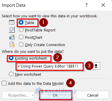
- Click Close & Load >> select Close & Load To.
- In Import Data, select Table.
- Select Existing worksheet and enter B11 in the box.
- Click OK.
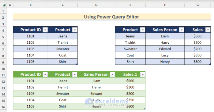
This is the output.
Read More: How to Combine Two Tables Using Power Query in Excel
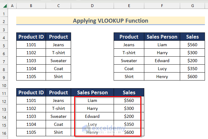
Method 2 – Left Join Applying the Excel VLOOKUP Function
Steps:
- Select B4:C9 and press Ctrl + C.
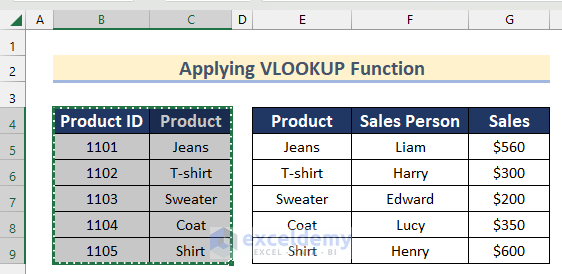
- Select B11 and press Ctrl + V.
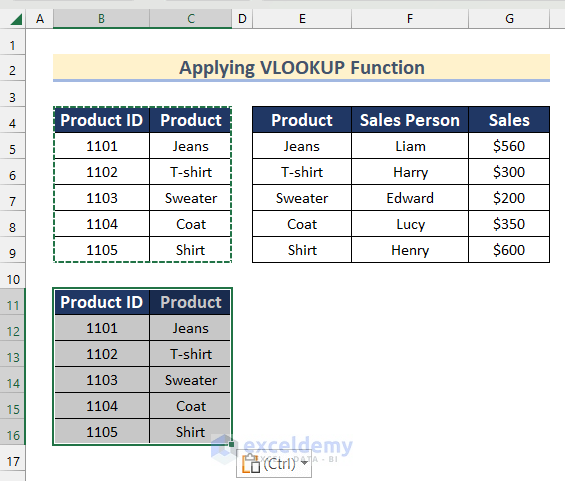
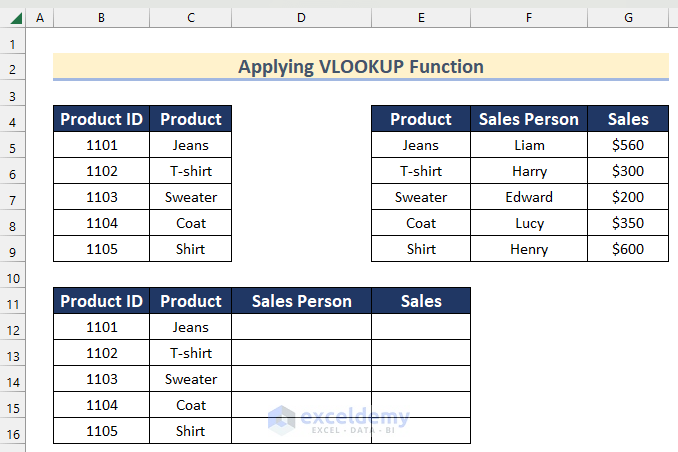
- Add the Sales Person and Sales columns to the copied dataset.
- Select D12 and enter the following formula.
=VLOOKUP(C12,$E$5:$G$9,{2,3},FALSE)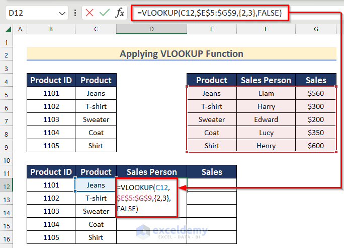
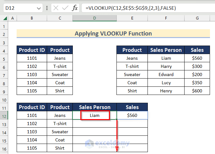
- Press Enter, and you will see the value of both Sales Person and Sales.
- Drag down the Fill Handle tool to autofill the formula.
In the VLOOKUP function, C12 is the lookup_value, E5:G9 is the table_array, 2 & 3 is col_index_num, and FALSE is range_lookup.
This is the output.
Read More: How to Perform Left Outer Join in Excel
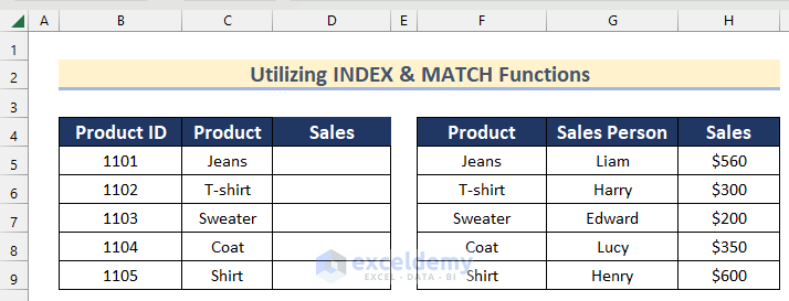
Method 3 – Utilize the INDEX & MATCH Functions to Left Join in Excel
Steps:
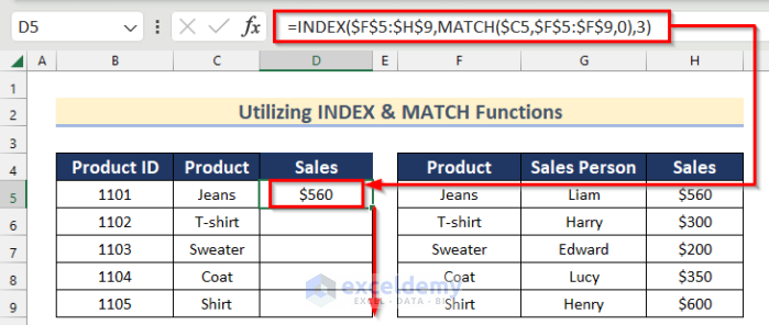
- Enter the following formula in D5.
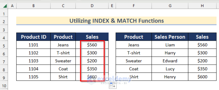
=INDEX($F$5:$H$9,MATCH($C5,$F$5:$F$9,0),3)- Press Enter and drag down the Fill Handle to autofill this formula.
Formula Breakdown
- MATCH($C5,$F$5:$F$9,0): The MATCH function returns the location of a lookup value. The Output is {1}.
- INDEX($F$5:$H$9,MATCH($C5,$F$5:$F$9,0),3): The INDEX function returns a cell value of a lookup value. The formula becomes INDEX($F$5:$H$9,1,3). Here, the Output is {560}.
- The Sales column is added to the first table.
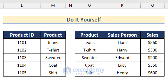
Practice Section
Practice here.
Download Practice Workbook
Download the workbook.
Related Articles
- How to Inner Join in Excel
- How to Perform Outer Join in Excel
- How to Create Full Outer Join in Excel
- How to Create Cross Join in Excel
<< Go Back to Power Query Excel | Learn Excel
Get FREE Advanced Excel Exercises with Solutions!
