Latest Posts From Arin Islam

This is an overview. Download Excel Workbook Data for Chart.xlsx How to Add a Chart in Excel The sample dataset contains the number ...

Note: In Excel 2016 or newer versions, you can directly insert a statistic chart. In older versions, you can use Data Analysis ToolPak or different ...
In this Excel tutorial, you will find ways to calculate Standard Deviation using different arithmetic formulas in Excel. Here, we'll discuss how you can ...

This is an overview Download Practice Workbook Student Info.xlsx Marksheet.xlsx Excel Components 1. Cells A cell in a ...

This is an overview: Download Practice Workbook Use of Date Range.xlsx How to Create a Date Range in Excel The dataset below contains ...

This is an overview: Click here to enlarge this image. Download Practice Workbook Date Format.xlsx The Date Format in Excel Dates in ...

In this Excel tutorial, we will discuss various ways to convert text to number format, including using Error Checking, Paste Special, Text to Columns and ...

Looking for ways to sort worksheets numerically using VBA in Excel? Then, this is the right place for you. Excel VBA can be used to automate numerous tasks, ...

1. Use StrPtr Function & If ElseIf Statement to Show If User Clicked Cancel Button in VBA Inputbox Insert the following code into your module. ...

We can use conditional statements, error handling, and the "Exit that part" option to break an infinite loop in Excel VBA. What is an Infinite Loop ...
This is an overview: 3 variables in different data types were shown in a MsgBox. The VBA MsgBox Function Objective: The MsgBox function is used ...

Introduction to ISNUMBER Function Function Objective The ISNUMBER function checks whether the value of a cell is a number or not. Syntax ...
What Is Interpolation? Interpolation means predicting a value between two specific given data points using the dataset. Data can be linear or nonlinear and ...
The sample dataset contains a To Do list and values to find. Check if cells contain one of these values. Method 1 - Combine the IF, SUMPRODUCT, ...

Method 1 - Using the XLOOKUP Function to Check If a Cell Contains Text and Return the Value in Excel The sample dataset contains students' Names. You want to ...
- 1
- 2
- 3
- …
- 8
- Next Page »
See Our Reviews at


Hi EDD,
Thanks for your comment. Hiding the Formula bar and Ribbon are typically done on a per-workbook basis and aren’t usually carried over to other workbooks you open. However, when you hide Formula Bar and Ribbon from any specific worksheet of your workbook, they’ll be removed from all the other worksheets of that workbook.
You can follow a manual process to align the range in the center of the screen. To center align all the elements on the screen, select the whole range and press Ctrl + X to cut the total range. Here, for the Home page, we will cut cell range B1:H12.
Then, press Ctrl + V to paste it in the center of your screen.
Similarly, you have to cut and paste all the elements to the center and align them on the screen manually.
We hope this will solve your problem. Please let us know if you face any further problems.
Regards,
Arin Islam,
ExcelDemy
Dear Anthony Maviglia,
Thank you for your comment. Sometimes keyboard shortcuts may not work in Excel for several reasons. You can check an alternative solution below.
• If you want to select column A and B and then unhide them, first press Ctrl + G >> type A:B in the Reference box >> click on OK. This will select your hidden columns.
• Then, go to the Home tab >> click on Format >> click on Hide & Unhide >> select Unhide Columns option.
I hope this will help you to solve your problem. Please let us know if you have other queries.
Regards,
Arin Islam
ExcelDemy.
Dear Eugenia,
Thank you for your comment.
To ensure that the progress bar accurately reflects the progress of your macro, you can use the following modified code.
• Insert this code into your module.
Here, the Progress_Bar subroutine is called by the cmd_Click event. We used the (Counter1 / 1000) * 100 formula to calculate the progress of the macro execution as a percentage and set it as the value of StatusBas.
• Then, create a button in your worksheet >> right-click on it >> select Assign Macro.
• Assign the Progress_Bar named macro to that button.
Now, if you click on the button, It will show progress in the status bar.
We hope this will solve your problem. Please let us know if you face any further problems.
Regards,
Arin Islam,
ExcelDemy
Hello Amjad,
To use the same code but save it as an Excel file without formulas you need to have some minor changes in the code.
• To create a name for saving the new Excel file use the following code. Here, we changed the “.pdf” part to “.xlsx” as you want to save it as an Excel file instead of a PDF.
• Then, to select a folder for the file use the following code. Here, we changed the FileFilter to “Excel Files (*.xlsx), *.xlsx” for the Excel file.
• Finally, save the worksheet as an Excel file using the following code. Here, we used the ActiveSheet.UsedRange.Value property which will copy only the values in the used range.
• After employing these changes, your code may look like the following one.
We hope this will solve your problem. Please let us know if you face any further problems.
Regards,
Arin Islam,
ExcelDemy
Hi FADYA,
Thanks for your appreciation.
When we auto-populate Word documents from Excel it automatically generates data in individual documents for each data.
However, you can go to the View tab and then click on Web Layout from the Views group to see all the values in a single layout.
Hi OZZY,
Thanks for your comment.
If the given codes are not working for the .Send function,
• Use the following code in your worksheet by clicking on View Code.
• Then, use the following code in your Module.
We hope this will solve your problem. Please let us know if you face any further problems.
Regards,
Arin Islam,
ExcelDemy
Hi KARL,
Thanks for your comment.
To always return 8 digits with a fill of 0 on the left side of the data you can use VBA code. Follow the steps given below to do that.
Steps:
• Firstly, go to the Developer tab >> click on Visual Basic.
• Then, it will open Microsoft Visual Basic for Applications.
• Now, open Insert >> select Module.
• Next, a Module will open then type the following code in the opened Module.
• Finally, Save the code and go back to the worksheet.
• Then, select the cell or cell range to apply the VBA.
• Here, we selected the range B5:B7.
• Next, open the Developer tab >> select Macros.
• After that, select Alphanumeric and click on Run.
• Thus, Excel will always return 8 Alphanumerics with a fill of 0 on the left side of the data string.
We hope this will solve your problem. Please let us know if you face any further problems.
Regards,
Arin Islam,
ExcelDemy
Hi MAHESWARI,
Thank you for your comment.
To create a leave record for 2023 in Excel you can follow the steps given in the article with some little changes.
• First of all, insert 1-Jan-2023 and 1-Feb-2023 in Cell E5 and E6.
• Then, drag the icon until it reaches the desired month. Here, we will drag until 1-Dec-23 for illustration.
• Next, you will get the following result.
• After that, follow the same steps shown in the article and you will be able to create a leave record for 2023.
We hope this will solve your problem. Please let us know if you face any further problems.
Regards,
Arin Islam,
ExcelDemy
Hello MRRRR,
Thank you for your comment. If you follow the first method, we have shown you will get the week number from a date according to the calendar.
• Here, to find the week number of 4th September 2021 we used the following formula and got 1 as the week number.
=WEEKNUM(B3,1)-WEEKNUM(DATE(YEAR(B3),MONTH(B3),1),1)+1• On the other hand, using the same formula we got 2 as the week number for 5th September 2021.
Hope you have found your solution. If you face any further problems, please share your Excel file with us at [email protected].
Regards
Arin Islam,
Exceldemy.
Hello ABC,
Thanks for your comment. No, there is no such limit to merging data. This code should perfectly work for the 5th sheet too. However, there are a limit for row (1,048,576) & column (16,384) numbers in Excel. If after merging the 5th sheet your data crosses this limit, it may not work.
Hope you have found your solution. If you face any further problems, please share your Excel file with us at [email protected].
Regards
Arin Islam,
Exceldemy.
Hello RALF,
Thanks for your comment. I suppose you are mentioning the first method. Here, we have shown you how to sort a single column. We have sorted only the column which contains the Age and the other column values (Name, Date of Birth) remained the same. That’s why after sorting the age changed for Amy Bryne.
If you have any other suggestions or face any problems, please share them with us in the comment section.
Regards,
Arin Islam
Exceldemy.
Hello Meni Porat,
Thanks for your kind suggestions.
Your formula may show a #VALUE error for an 8-digit number.
However, removing +0 from the formula will return the correct result.
If you have any other suggestions or face any problems, please share them with us in the comment section.
Regards
Arin Islam,
Exceldemy.
Hello, MELVIN MORALES!
Thanks for your comment. You can click here to autoscroll and you’ll find the download links for both pdf and xlsx formats.
https://www.exceldemy.com/microsoft-excel-formulas-functions-cheat-sheet/#Download_Excel_Formulas_Cheat_Sheet_PDF
Regards
Arin Islam,
Exceldemy.
Hi RC GOYAL,
Thanks for your feedback.
In the formula, we used {0,0} in the combination formula to return a two column array. However, you can avoid it for this dataset. It will return the same result.
If you face any further problems, please share your Excel file with us at [email protected].
Regards
Arin Islam,
Exceldemy.
Hello HBING,
To solve your issue follow the steps given below.
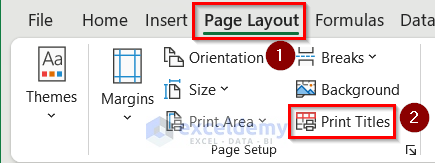
• Firstly, go to the Page Layout tab >> click on Print Titles.
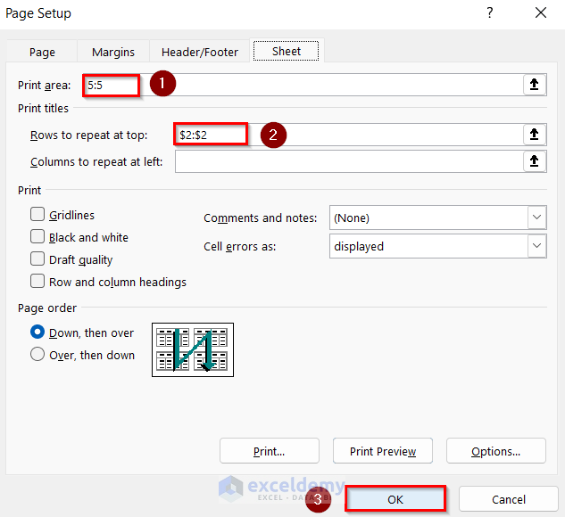
• After that, type 5:5 as Print Area and $2:$2 as Rows to repeat at top.
• Then, click on OK.
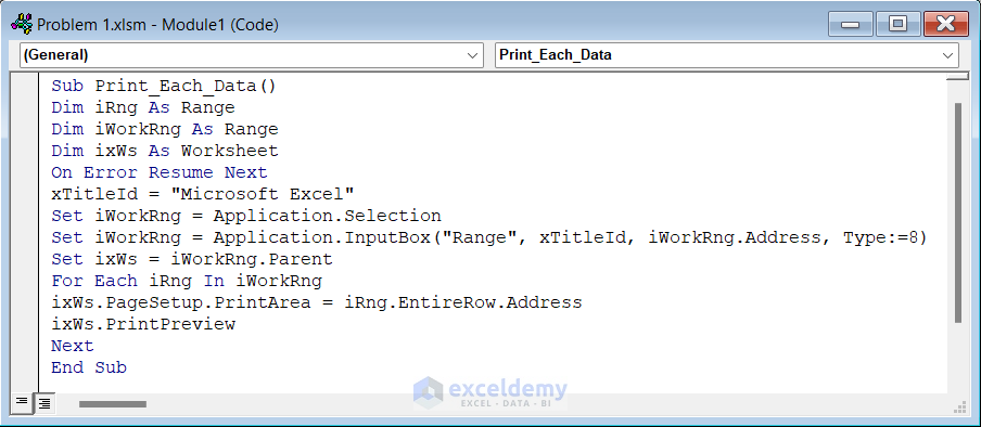
• Now, write the following code in your module.
Sub Print_Each_Data()
Dim iRng As RangeDim iWorkRng As RangeDim ixWs As WorksheetOn Error Resume NextxTitleId = "Microsoft Excel"Set iWorkRng = Application.SelectionSet iWorkRng = Application.InputBox("Range", xTitleId, iWorkRng.Address, Type:=8)Set ixWs = iWorkRng.ParentFor Each iRng In iWorkRngixWs.PageSetup.PrintArea = iRng.EntireRow.AddressixWs.PrintPreviewNextEnd Sub• Next, click on Macros from the Developer tab.
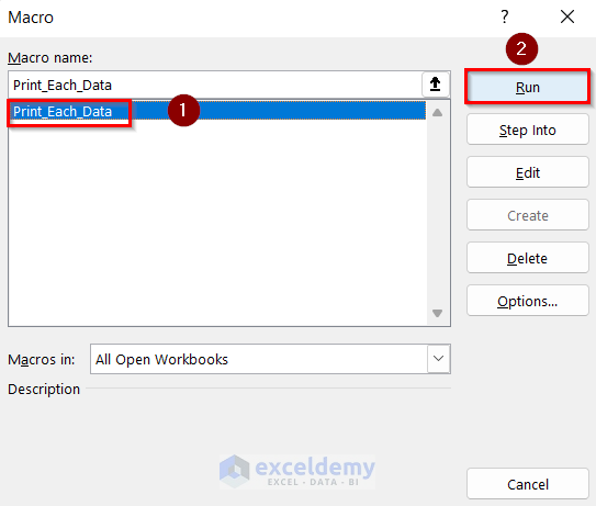
• Select the macro named Print_Each_Data.
• Lastly, click on Run.
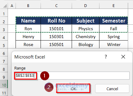
• Now, a box will open.
• Then, select the range which you want to print. Here, we selected cell range B2:E3.
• Finally, click on OK.
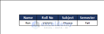
• Thus, you can print each student’s data automatically in the same format.
If you face any further problems, please share your Excel file with us in the comment section.
Regards
Arin Islam,
Exceldemy.
Hello AMGHAR,
Thanks for your feedback.
If you face any further problems, please share your Excel file with us in the comment section.
Regards
Arin Islam,
Exceldemy.
Hello Lodewijk,
I suppose you want to know more about the Power Query Editor and how it can add sheets to get unique values.
Power Query Editor is very useful in the case of data preparation.
To use this editor, you have to use the Get Data feature from the Data tab. You can get data from different kinds of files such as Excel workbooks, PDFs, Text, etc. Then, you can transform those datasets using the operator available. Here, we removed rows from the tables. You can also combine different tables from those files by the Append or Merge operator. The Append operator is used to create a new query having all the rows from the datasets and the Merge operator is used to have a query with all the columns. You have to use the Append operator to get the unique values. Finally, you can load the query in the existing worksheet or a new worksheet.
If you face any further problems, please share your Excel file with us in the comment section.
Regards
Arin Islam,
Exceldemy.
Hello ANANDA,
#NAME error mostly occurs when you misspell the function name. Please check if you have used the correct spelling of the function.
There can be another reason behind this. If you notice you will see that W had fixed the Cell value in the COUNTIF function which is used as the range. Try to use only Cell J2 as the range without making it a fixed range.
If you are using Excel 365 version you only need to press Enter after inserting this array formula. But, for previous versions press Ctrl+Shift+Enter.
I hope that your problem will be solved now.
If you face any further problems, please share your Excel file with us in the comment section.
Regards
Arin Islam
Hi Mohammed Shahid,
You can pull text from multiple sheets and ignore blank or space by using the TRIM function. This function will help you to remove space automatically.
To solve your problem, use the following formula in Cell B2 of Sheet 3 in your Excel worksheet.
=TRIM(Sheet1!B2&" "&Sheet2!B2)Hope this will solve your problem. Feel free to comment if you have further inquiries.
Regards,
Arin Islam.
Greetings LIBBY,
Thank you for letting us know. We’ve updated it.
Feel free to comment if you have further inquiries. We are here to help.
Regards
Arin Islam (Exceldemy Team)
Hi Sue,
Hope you are doing well.
You can approximately match addresses on 2 sheets and find a job associated with that address.
Here, we created a dataset in Sheet1 according to your description.
Again, this is Sheet2 containing the exact Address and Job record.
Now, to approximately match addresses on 2 sheets and find a job associated with that address use the formula given below in Sheet1 Cell C5.
=VLOOKUP(B5,Sheet2!$B$5:$C$11,1,TRUE)Thanks.
Regards,
Arin Islam
Hi Colin Kinsella,
Hope you are doing well.
You can select multiple columns from A to Z having different lengths.
Here, we created a dataset in Cell range A4:Z6. Then, we selected Cell B4:E4 similar to your dataset.
After selecting Cell range B4:E4 or any other cells, press CTRL+A on your keyboard to select all remaining rows with data.
Thanks.
Regards,
Arin Islam
Hi J,
Hope you are doing well.
You can get the actual numerical difference between two cells by using subtraction (-) in the formula. In case of, percentage value use the formula given below.
=IF(AND(0<D5,D5<$D$10),(D5/$D$10)*100&"% Less Than 10",(-D5/$D$10)*100&"% Greater Than 10")If the condition is True then the formula will return the result as follows.
On the other hand, if the condition is False then the formula will return the result as follows.
Here, the AND function will return True if both the conditions are true else it will return False.
Thanks.
Regards,
Arin Islam