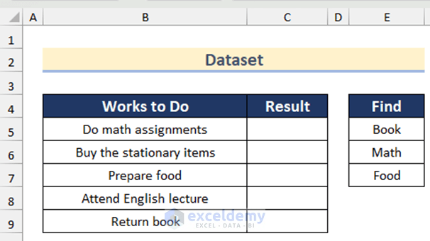
The sample dataset contains a To Do list and values to find.
Check if cells contain one of these values.
Method 1 – Combine the IF, SUMPRODUCT, ISNUMBER & SEARCH Functions to Check If a Cell Contains One of Several Values
Steps:
- Select C5 and enter the following formula.
=IF(SUMPRODUCT(--ISNUMBER(SEARCH($E$5:$E$7,B5))),"Yes","No")- Press Enter.
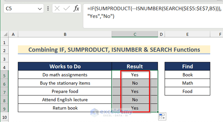
- Drag down the Fill Handle to see the result in the rest of the cells.
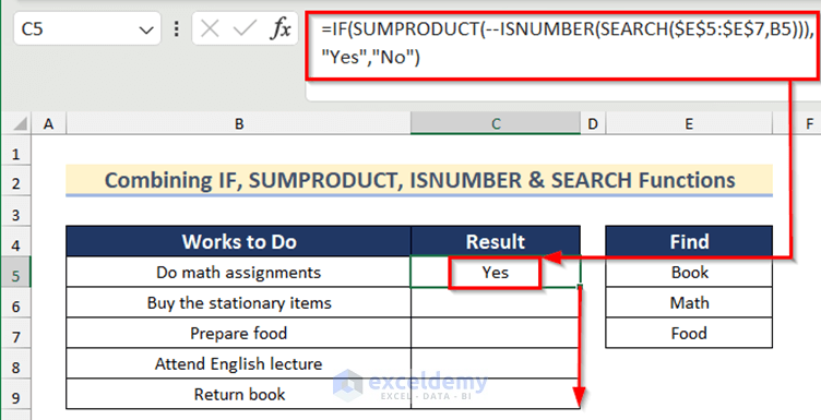
- You will get Yes or No as a result.
Formula Breakdown
- The SEARCH function searches cell range E5:E7 in B5.
- The ISNUMBER function checks if the result is a number.
- The SUMPRODUCT function adds those numbers.
- The IF function returns “Yes” if the resultant of the SUMPRODUCT function is greater than 0. Otherwise, “No”.
Read More: How to Use IF Statement with Yes or No in Excel
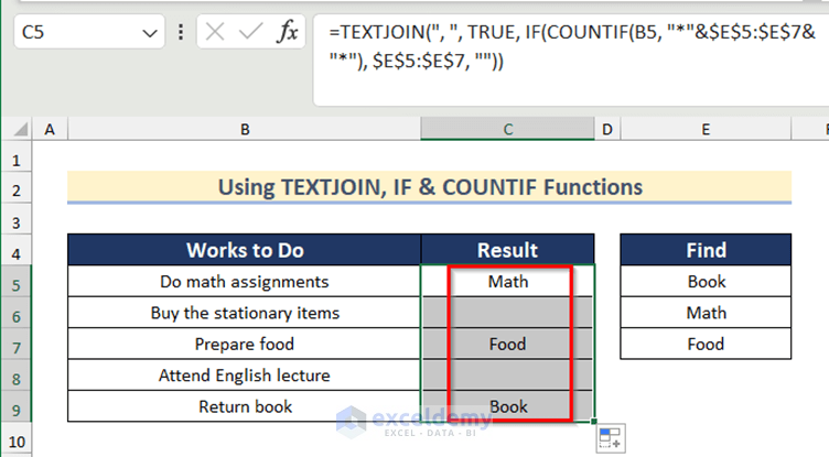
Method 2 – Check If Cell Contains One of Multiple Values Using TEXTJOIN, IF & COUNTIF Functions Together
Steps:
- Select C5 and enter the following formula.
=TEXTJOIN(",",TRUE,IF(COUNTIF(B5,"*"&$E$5:$E$7&"*"),$E$5:$E$7,""))- Press Enter.
- Drag down the Fill Handle to see the result in the rest of the cells.
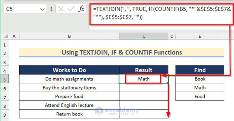
This is the output.
Formula Breakdown
- The COUNTIF function counts the number of values in B5 in E5:E7.
- The IF function returns the value or return Blank if not found.
- The TEXTJOIN function joins the found values. Here, comma (,) is used as delimiter.
Read More: How to Prepare IF Statement Contains Multiple Words in Excel
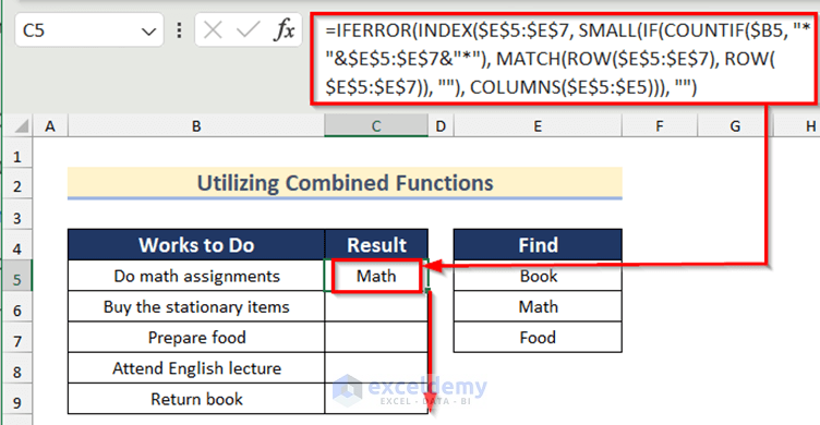
Method 3 – Utilize Combined Functions to Find If Cell Contains One of Several Values
Steps:
- Select C5 and enter the following formula.
- and press Enter.
=IFERROR(INDEX($E$5:$E$7,SMALL(IF(COUNTIF($B5,"*"&$E$5:$E$7&"*"),MATCH(ROW($E$5:$E$7),ROW($E$5:$E$7)),""),COLUMNS($E$5:$E5))),"")
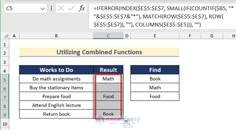
- Drag down the Fill Handle to see the result in the rest of the cells.
This is the output.
Formula Breakdown
- The ROW function finds the row number of E5:E7.
- The COLUMNS function calculates the number of columns in the given range.
- The COUNTIF function counts the number of values present in B5 in E5:E7.
- The MATCH function returns the relative position of E5:E7.
- The result of the COUNTIF function is used as logical_test, the result of the MATCH function as value_if_true and Blank as value_if_false in the IF function.
- The SMALL function returns the result of the IF function as array and the result of the COLUMNS function as k.
- In the INDEX function E5:E7 is used as array and the result of the SMALL function as row_num.
- The IFERROR function is used to avoid errors and returns Blank if there is an error.
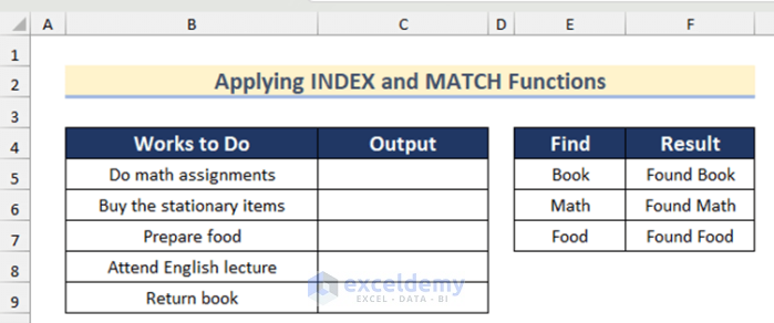
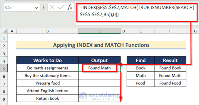
Method 4 – Applying INDEX and the MATCH Functions to Check If Cell Stores One of Several Values in Excel
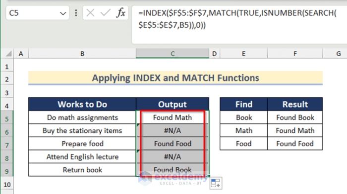
A #N/A error is displayed for the cells that do not contain any of the values you are looking for.
Steps:
- Select C5 and enter the following formula.
=INDEX($F$5:$F$7,MATCH(TRUE,ISNUMBER(SEARCH($E$5:$E$7,B5)),0))- Press Enter.
- Drag down the Fill Handle to see the result in the rest of the cells.
This is the output.
Formula Breakdown
- The SEARCH function searches E5:E7 in B5.
- The ISNUMBER function checks if the result of the SEARCH function is a number.
- In the MATCH function, TRUE is used as lookup_value, the result of ISNUMBER function as lookup_array and 0 as match_type.
- In the INDEX function, F5:F7 is used as array and the result of the MATCH function as row_num.
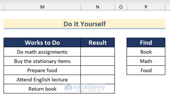
Practice Section
Practice here.
Download Practice Workbook
Download the workbook.
Related Articles
- How to Use Conditional Formatting If Statement Is Another Cell
- Excel IF Statement Between Two Numbers
- How to Find Sum If Cell Color Is Green in Excel
- Use Wildcard with If Statement in Excel
- Show Cell Only If Value Is Greater Than 0 in Excel

