Download the Practice Workbook
Why Wildcard with IF Statement Is Not Working
Consider the following function.
=IF(C5= "*a*", "Match", "Not Match")The formula doesn’t give you the output you wanted. You can see this formula is showing “Not Match” even if there is an “a” in the IDs.
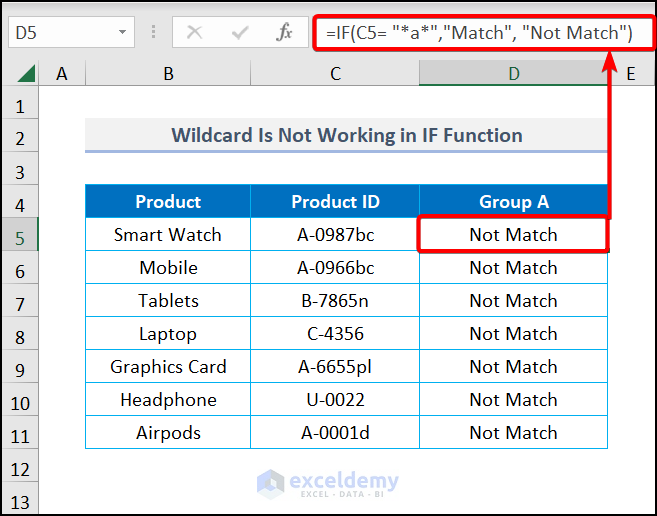
Excel can’t recognize wildcards matched with an equal sign or any other operators.
5 Methods to Use Wildcard with IF Statement in Excel
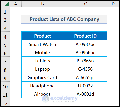
You can’t use the wildcard in the IF formula alone, but you can use it in conjunction with other functions. We’ll use a dataset of Product Lists of ABC Company. We will look for a specific partial text with the wildcards.
Method 1 – Using IF and COUNTIF Functions for Wildcards
Steps:
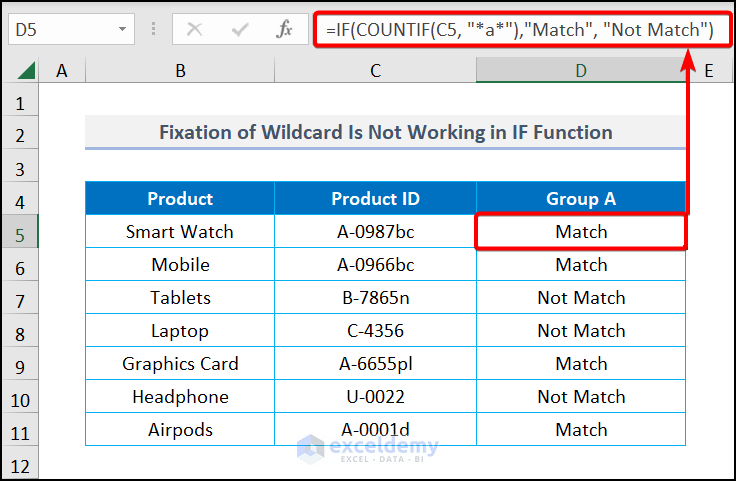
- Go to cell D5 and insert this formula:
=IF(COUNTIF(C5, "*a*"), "Match", "Not Match")- AutoFill to the other cells in the column.
The COUNTIF function is used as the logical_test for the IF function. The function takes the value of cell C5 and matches it with “*a*”. It returns 1 for a match and 0 for not matching. The IF function takes 1 as TRUE, and 0 as FALSE. The IF function then displays “Match” for TRUE and “Not Match” for FALSE.

Read More: How to Check If Cell Contains One of Several Values in Excel
Method 2 – Utilizing COUNTIF and OR Functions
Steps:
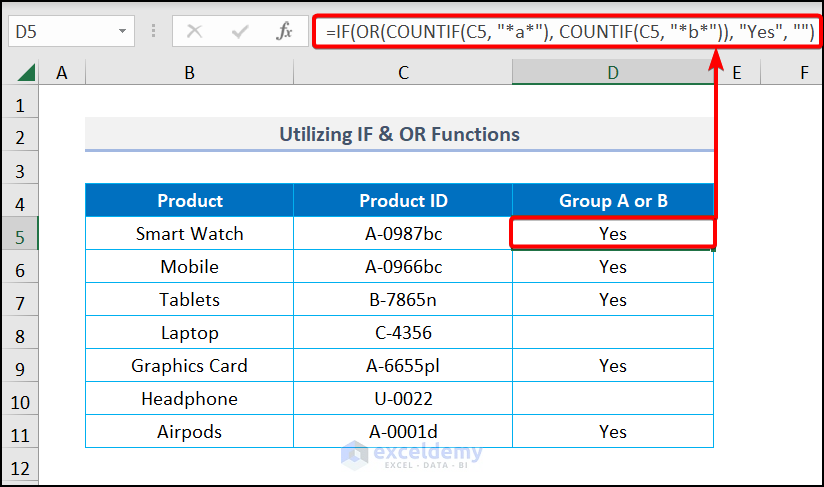
- Go to cell D5 and insert the following formula:
=IF(OR(COUNTIF(C5, "*a*"), COUNTIF(C5, "*b*")), "Yes", "")If you want to find two different partial matches, you need to use the OR function to make two separate COUNTIF checks.
- Press Enter and drag down to get the following output for other cells.
Read More: How to Use IF Statement with Yes or No in Excel (3 Examples)
Method 3 – Applying ISNUMBER and SEARCH Functions
The SEARCH function returns the relative position of the argument. Then the ISNUMBER function returns the value in binary order. So it takes the partial text as its logical value. The procedure for using this formula is stated below.
Steps:
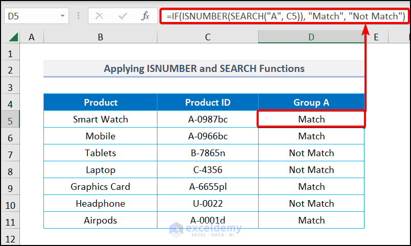
- In cell D5, insert the following formula, apply it, and AutoFill through the column.
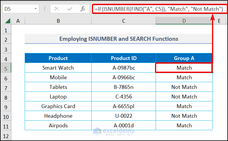
=IF(ISNUMBER(SEARCH("A", C5)), "Match", "Not Match")Formula Breakdown:
- SEARCH(“A”, C5)searches for the letter “A” in cell C5 and returns the relative position of the letter.
- ISNUMBER(SEARCH(“A”, C5)) returns the logical TRUE if it finds “A” in cell C5 and vice-versa.
- The returned value is then used as the logical_test of the IF formula. If the text is TRUE, it displays “Match”. If the text is FALSE, it displays “Not Match”.
Similar Readings
- How to Use Multiple IF Statements in Excel Data Validation
- How to Use If Statement Based on Cell Color in Excel (3 Examples)
- Dynamic Data Validation List in Excel with IF Statement Condition
- How to Use IF Statement with Not Equal To Operator in Excel
Method 4 – Employing ISNUMBER and FIND Functions
Steps:
- Go to cell D5, insert this formula, apply it, and AutoFill the column.
=IF(ISNUMBER(FIND("A", C5)), "Match", "Not Match")Formula Breakdown:
- FIND(“A”, C5) finds the letter “A” in cell C5 and returns the relative position of the letter.
- ISNUMBER(SEARCH(“A”, C5)) returns the logical TRUE if it finds “A” in cell C5 and vice-versa.
- The returned value is then used as the logical_test of the IF formula. If the text is TRUE it displays “Match”.
Method 5 – Incorporating IF and AND Functions
Steps:
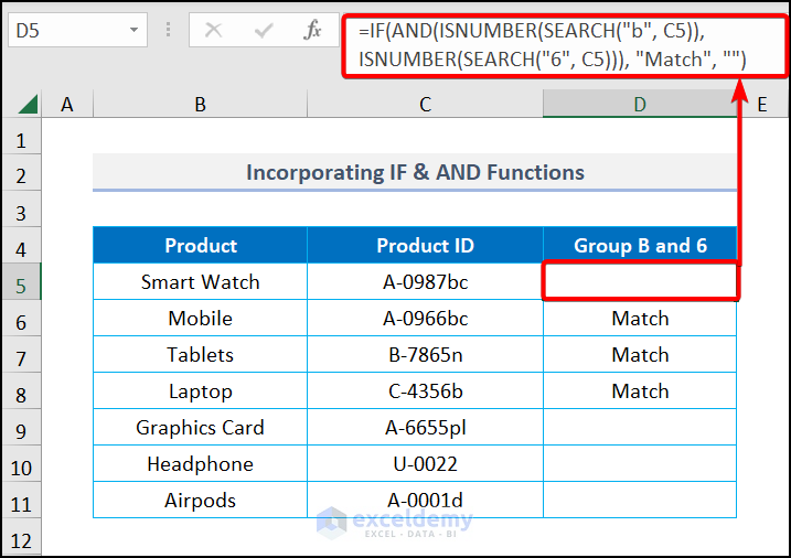
- Go to cell D5 and input the formula, then use AutoFill for the column.
=IF(AND(ISNUMBER(SEARCH("b", C5)), ISNUMBER(SEARCH("6", C5))), "Match", "")The AND function joins the results returned by the ISNUMBER and the SEARCH functions. The IF formula takes the returned value as logical_test. When the logical_test argument is TRUE, it displays “Match“. When the value is FALSE, it remains blank.
Read More: How to Use IF Function with OR and AND Statement in Excel
What to Do If Wildcard with IF Statement Is Not Working?
- Use a wildcard as a part of a string in a formula that compares strings, such as COUNTIF:
=IF(COUNTIF(C5, "*a*"), "Match", "Not Match")The COUNTIF function counts for the letter “a” inside wildcard asterisks (*). Then, the IF function takes the output of the COUNTIF function as a logical_test and returns “Match” if the argument meets the criteria. Otherwise, It returns “Not Match”. See the image below for a better understanding.
Practice Section
We have provided a practice section on each sheet on the right so you can practice with different datasets and formulas.
Related Articles
- Use Conditional Formatting If Statement Is Another Cell
- Excel IF Statement Between Two Numbers (4 Ideal Examples)
- Find Sum If Cell Color Is Green in Excel (4 Easy Methods)
- How to Prepare IF Statement Contains Multiple Words in Excel
- Show Cell Only If Value Is Greater Than 0 in Excel (2 Examples)


Brilliant. I liked all of your methods, but the COUNTIF function solved my problem. I used it with nested conditionals for keyword searches to categorize annual income and expenses from a download of bank transactions. It saved me a lot of time.
Hello Wade Kellogg,
Thank you for your feedback and appreciation. It is kind of you! I’m glad you found the COUNTIF function helpful for categorizing income and expenses from your bank transactions. It’s fantastic to hear that it saved you time. Happy Excel-ing!
Regards
ExcelDemy