Conditional Formatting is an excellent feature to format your worksheet based on specific criteria. For instance, you can use Conditional Formatting to highlight cells that have specific values. The cell value can be above or below the predetermined threshold or contain a particular text or date. However, this article will demonstrate to you how to use conditional formatting if a statement is another cell in Excel.
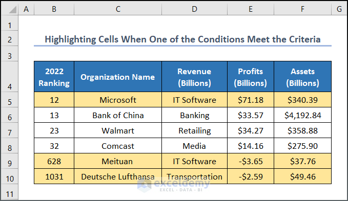
The image given below is an overview image and depicts the use of conditional formatting if the statement is another cell in Excel.
2 Relevant Cases to Use Conditional Formatting If Statement Is Another Cell in Excel
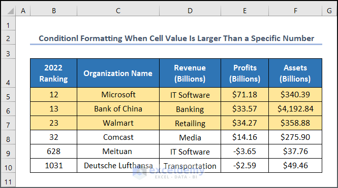
Let’s assume we have a dataset, namely “Forbes Listed Top Company”. You can use any dataset suitable for you.
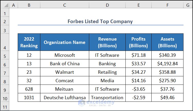
Here, we have used the Microsoft Excel 365 version; you may use any other version according to your convenience.
1. Using Conditional Formatting on Single Condition
Excel provides multiple ways to set a prerequisite condition to format your cell. The condition can be applied depending on the type of your task. You can highlight a specific cell that contains similar data, greater than, or less than your preset value. However, we are going to show some of the practical cases by which you can understand how this feature work. So, to apply Conditional Formatting to a single condition in Excel, follow the instruction we are going to provide below.
1.1 Conditional Formatting When Cell Value Is Larger Than Specific Number
📌 Steps:
- First of all, select the range of data you want to format. B5:F10 for instance.
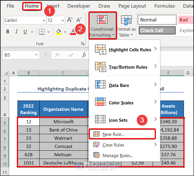
- Then, click on Home tab> Conditional Formatting feature> New Rule.
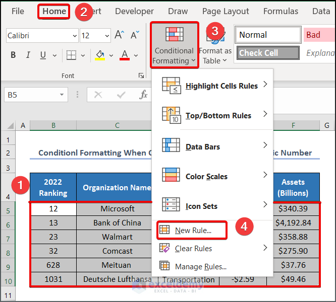
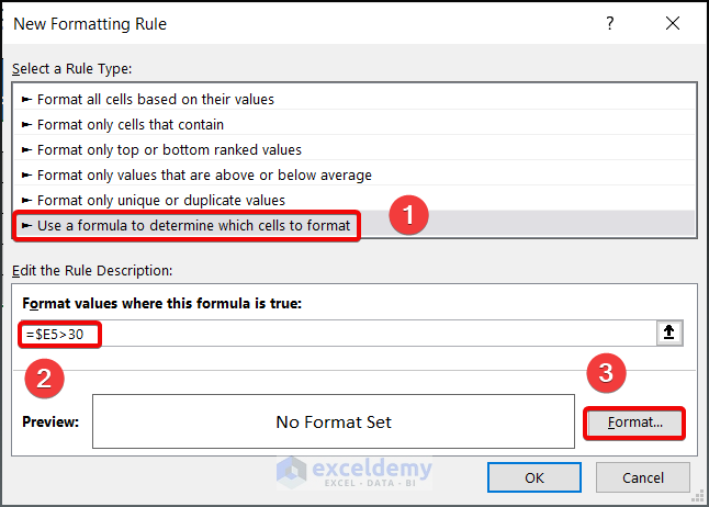
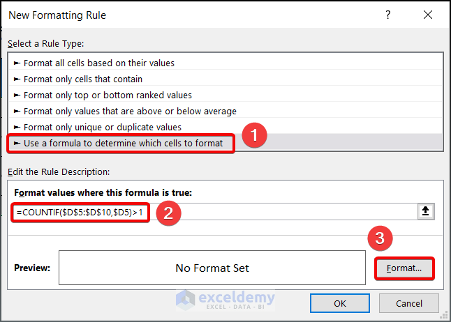
- In the dialog box that appears, choose to Use a formula to determine which cells to format.
- Enter the formula given below in the Format values where this formula is true box.
=$E5>30- Click Format button to add a highlighting color.
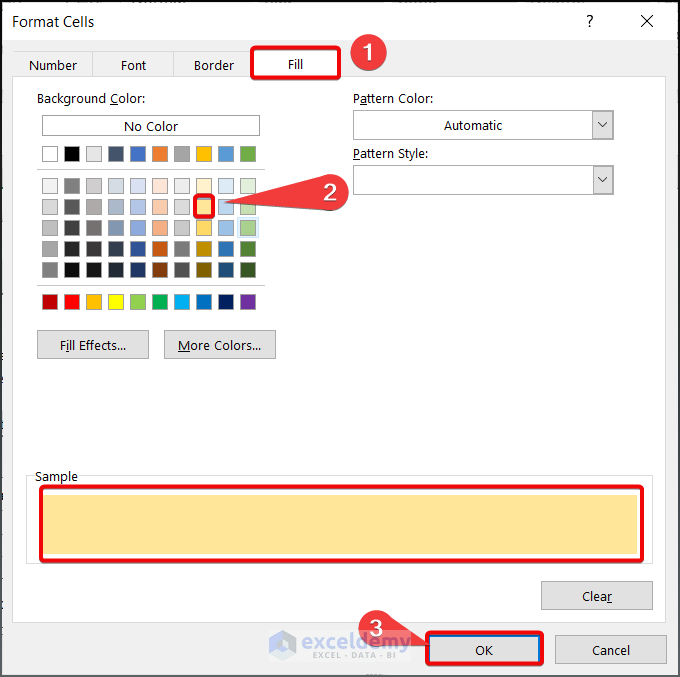
- Subsequently, another dialog box will appear.
- From Fill tab, select Gold Accent 4, Lighter 60% as your cell background color. However, you can choose any of the colors according to your preference.
- Then click OK.

- Following that, click the OK button to close the New Formatting Rule window.
- Now see the output of the given condition below.
Read More: How to Use If Statement Based on Cell Color in Excel
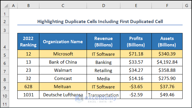
1.2 Highlighting Duplicate Cells Including First Duplicated Cell
If you want to highlight the duplicate values of your dataset, you can do this by using a predefined feature under Conditional formatting > Highlight Cells Rules > Duplicate Values.
However, if you want to highlight the entire row which contains the duplicate value, you can follow the demonstration we are going to describe below.
📌 Steps:
- Similar to the previous work, select the range B5:F10 which contains the data you want to format.
- Then, click on Home tab> Conditional Formatting feature> New Rule.
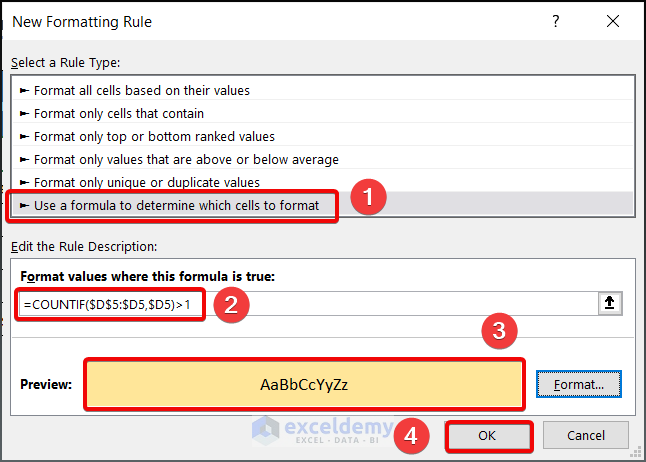
- Choose to Use a formula to determine which cells to format option from the appeared dialog box.
- Enter the formula given below the Format values where this formula is true box.
=COUNTIF($D$5:$D$10,$D5)>1- Click the Format button to add a highlighting color.
- From the appeared dialog box, select Fill tab >> Gold Accent 4, Lighter 60% as your cell background color. However, you can choose any of the colors according to your preference.
- Then, click OK.
- Press the OK button to close the dialog box.

- Thus the rows which contain duplicate data IT Software will be highlighted across the selected range. See the final output as given below.
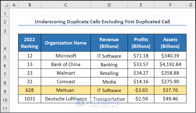
1.3 Underscoring Duplicate Cells Excluding First Duplicated Cell
To disregard the first event and highlight future duplicate values, you have to make a small change in your formula. Follow the instruction given below.
📌 Steps:
- As usual, select the range B5:F10 which contains the data you want to format.
- Then, click on Home tab> Conditional Formatting feature> New Rule.
- Choose to Use a formula to determine which cells to format option from the appeared dialog box.
- Enter the formula given below in the Format values where this formula is true box.
=COUNTIF($D$5:$D5,$D5)>1- Select Gold Accent 4, Lighter 60% color by clicking the Format button.
- Press OK afterward.
- Now see the output where the first row containing IT Software data has been ignored, rather than the second row has been highlighted.
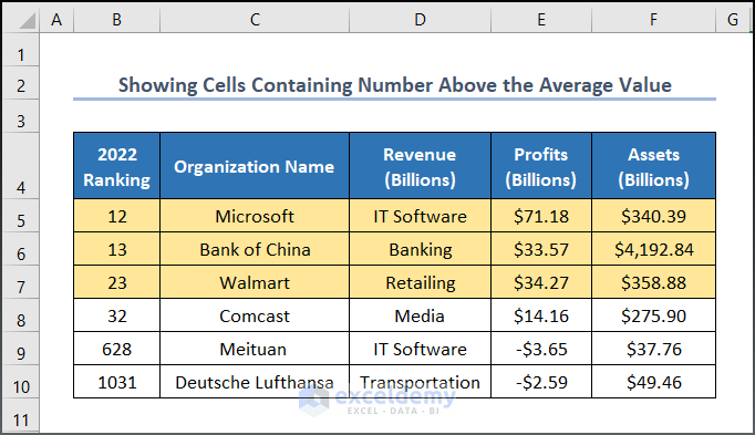
1.4 Showing Cells Containing Number Above Average Value
When you work with a bulk amount of data, the AVERAGE function may come as a handy function to employ in the conditional formatting formula bar. Thus it will highlight those value that contains greater, equal, or greater value than the average one depending on which criteria you would like to set. Here, we have used one case to demonstrate its utility.
📌 Steps:
- Select the range B5:F10 which contains the data you want to format.
- Then, click on Home tab> Conditional Formatting feature> New Rule.
- Click Use a formula to determine which cells to format the option from the appeared dialog box.
- Enter the formula given below in the Format values where this formula is true box.
=$E5>AVERAGE($E$5:$E$10)- Select Gold Accent 4, Lighter 60% color by clicking Format button.
- Press OK afterward.

- Thus you will have an output highlighting those rows that contain values more than the average value of the E column.
Read More: Show Cell Only If Value Is Greater Than 0 in Excel
2. Utilizing Conditional Formatting on Multiple Conditions
In Excel, you can use multiple conditions in conditional formatting. In the formula editor of the New Rule dialog box, you can enter a formula that uses logical operators (such as AND or OR) to combine multiple conditions. For example, if you want to apply formatting to cells in a range that are greater than 110 and less than 220, you can use the following formula:
=AND(A1>110,A1<220)This condition will work when both conditions are satisfied.
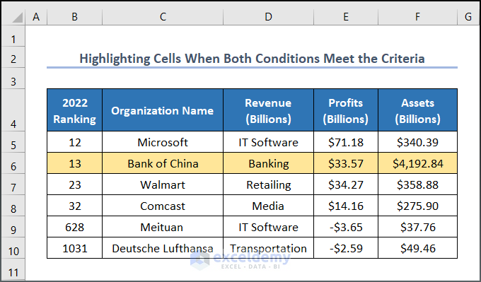
2.1 AND Function on Conditional Formatting When Both Conditions Meet Criteria
📌 Steps:
- Select the range B5:F10 which contains the data you want to format.
- Then, click on Home tab> Conditional Formatting feature> New Rule.
- Press Use a formula to determine which cells to format the option from the appeared dialog box.
- Enter the formula given below in Format values where this formula is true box.
=AND($D5="Banking",$E5>30)- Select Gold Accent 4, Lighter 60% color by clicking Format button.
- Press OK afterward.
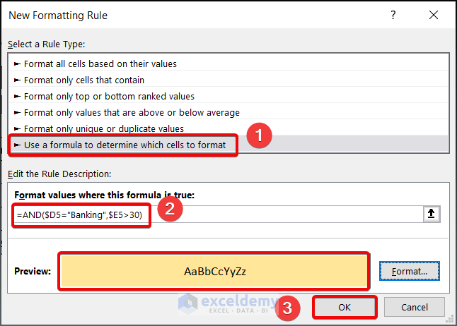
Now the logical operator AND function sort the data based on the condition. Thus the row that contains Banking as a string and has an E column value of more than 30 will be highlighted with the formatted color. see the output given below.
2.2 OR Function in Conditional Formatting While One of the Conditions Meet Criteria
Similarly, you can incorporate OR function to accomplish the task. In this way, the row will be highlighted if any of the preset conditions meet with cell value.
📌 Steps:
- Same old ritual, select the range B5:F10 where your data reside.
- Click on Home tab> Conditional Formatting feature> New Rule.
- Press Use a formula to determine which cells to format option from the appeared dialog box.
- Enter the formula given below in Format values where this formula is true box
=OR($E5>35,$E5<0)- Select Gold Accent 4, Lighter 60% color by clicking Format button
- Press OK afterward.
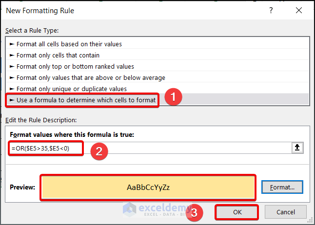
- Now see the output as given below.
Read More: How to Use IF Function with OR and AND Statement in Excel
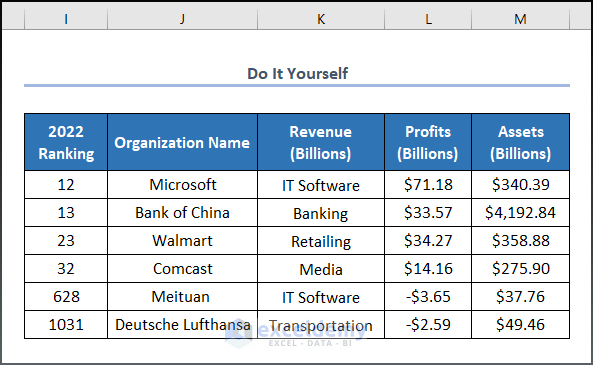
Practice Section
We have provided a Practice section on the right side of each sheet so you can practice yourself. Please make sure to do it yourself.
Download Practice Workbook
You can download and practice the dataset that we have used to prepare this article.
Conclusion
In this article, we have discussed how to use conditional formatting if a statement is another cell in Excel. As you have already understood, there are plenty of ways to do this task. So before inputting any specific formula in the New Formatting Rule dialog box, ensure the formula you choose aligns with your work. Further, if you have any queries, feel free to comment below and we will get back to you soon.
Related Articles
- How to Use If Then Else Statement in Excel VBA
- Excel IF Statement Between Two Numbers
- How to Find Sum If Cell Color Is Green in Excel
- Prepare IF Statement Contains Multiple Words in Excel
- How to Use Wildcard with If Statement in Excel
- Use IF Statement with Yes or No in Excel

