How to Use the AVERAGE Function in Excel (5 Examples)

Introduction to Excel AVERAGE Function

The AVERAGE function is categorized under the Statistical functions in Excel. This function returns the average value of a given argument.

Summary:

Returns the average (arithmetic mean) of its arguments, which can be numbers, names, arrays, or references that contain numbers.

Syntax:

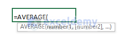
AVERAGE (number1, [number2], ...)

Arguments:

Argument	Required/Optional	Explanation
number1	Required	This is the first number, cell reference, or range for which we want the average.
number2	Optional	Additional numbers, cell references, or ranges for which you want the average, up to a maximum of 255.

Example 1 – Basic Use of the AVERAGE Function

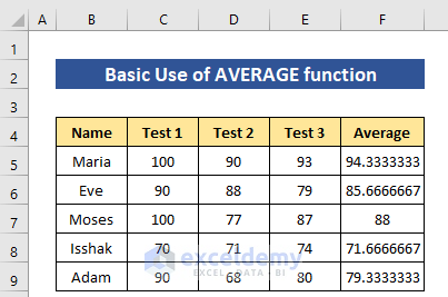
Suppose we have a simple dataset of five students and their scores in three tests. To find the average score for each student, insert the following formula in cell F5:

=AVERAGE(C5:E5)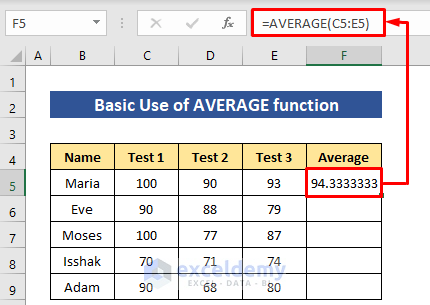

Basic Use of AVERAGE Function

Press Enter.
Replace the cell references as needed to find averages for other students.
Or use the Fill Handle tool to copy the formula down to the other cells in column F.

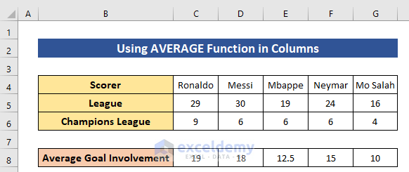
Use AVERAGE Function in Columns

If you have a dataset of scorers and their goals in different leagues, you can find the average goal involvement. For example, to find the average goal involvement of player Ronaldo (in cell C8):

=AVERAGE(C5:C6)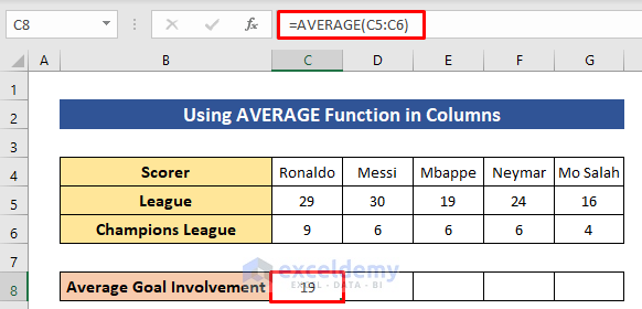

Use AVERAGE in Columns

We have calculated the average goal involvement of Ronaldo.
Use the Fill Handle tool to copy the formula across to obtain the result for the rest of the players.

Example 2 – Find the Average Percentages

If you need to find the average of percentage values, use the AVERAGE function.

For a range like C5:C9 containing score percentages enter the following formula in cell C11 and press Enter to get the result:

=AVERAGE(C5:C9)

Find the Average of Percentage

Example 3 – Calculating the Average Time

To calculate the average time from a dataset of marathon racers’ finishing times (formatted as h:mm:ss), enter the following formula in cell C11:

=AVERAGE(C5:C9)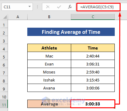

Find the Average of Time

The formula has produced the average time, and the format remains as the source time.

Example 4 – Average of the Top N Values

Suppose you want to find the average of the top 3 test scores.

Combine the LARGE and AVERAGE functions in cell H5:

=AVERAGE(LARGE(C5:G5,{1,2,3}))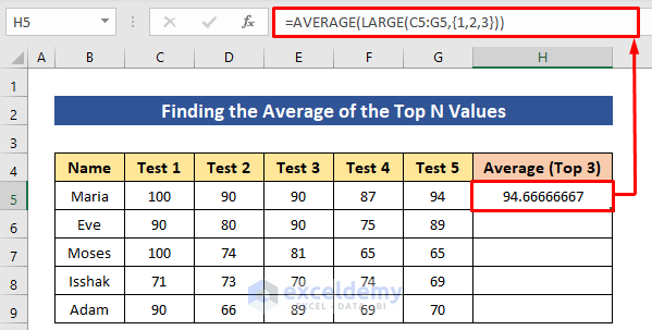

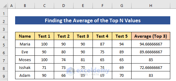
Find the Average of the Top N Values

The LARGE function returns the highest 3 values, and then AVERAGE computes their average.

Next, apply the Fill Handle tool to copy the formula to the other cells.

Note: If you need to find the average of n number of least values you can use SMALL in place of LARGE.

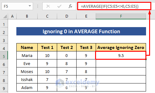
Example 5 – Find Average Ignoring 0

Sometimes your dataset may contain zeros, but you want to calculate the average while excluding those zeros. In such cases, you can combine the IF function with the AVERAGE function. Here’s how:

Suppose you have a dataset in cells C5:E5, and you’ve inserted a zero in cell D5.
To find the average of the non-zero values, use the following formula in cell F5:

=AVERAGE(IF(C5:E5<>0,C5:E5))

Press Enter, and you’ll get the average, ignoring the zeros.

How to Ignore 0 in Excel AVERAGE Function

Formula Breakdown:

IF(C5:E5<>0, C5:E5): The IF function returns the range excluding zero values.
AVERAGE(IF(C5:E5<>0, C5:E5)): The AVERAGE function then calculates the average for this modified range.

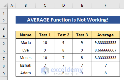
How to Solve it When Excel AVERAGE Function Is Not Working

Sometimes you might encounter issues with the AVERAGE function. For example, if you see a #DIV/0! error, it could be due to the following reason:

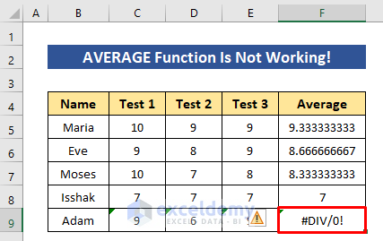
AVERAGE Function Is Not Working in Excel

Text Format: If the numbers in a row are stored as text (instead of numeric values), the AVERAGE function won’t work correctly.

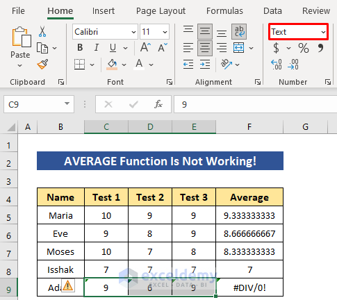
Chnage Format When AVERAGE Function Is Not Working in Excel

Solution:

Select the numbers.
Click on the error icon.
Choose the Convert to Number option from the menu.

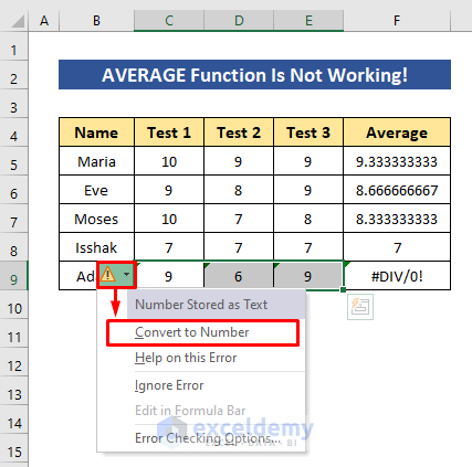
Use Convert to Number Option When AVERAGE Function Is Not Working in Excel

The average formula will now work.

Quick Notes

You can provide numbers directly alongside cell references.

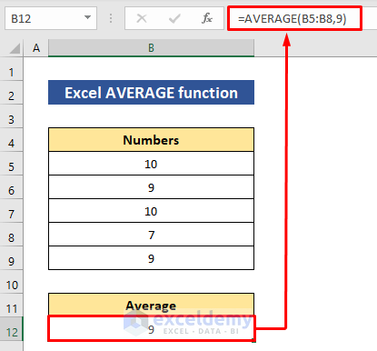
For instance, if you insert the number 9 with cell references B5 through B8 (containing 10, 9, 10, and 7), you’ll find the average.

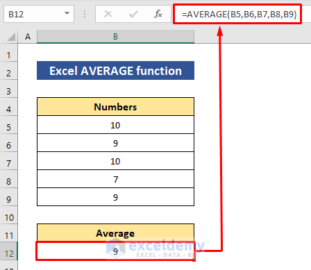
Besides using a range, you can set multiple cell references separated by commas within the AVERAGE function.

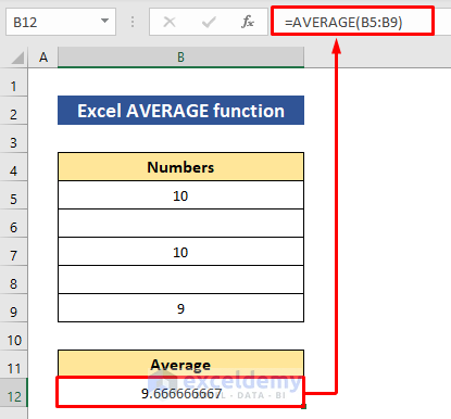
The AVERAGE function can handle empty cells within the provided range; it ignores them and calculates the average for the remaining cells.

Here we have provided B5 to B9 and B6 and B8 are empty cells. The AVERAGE function will ignore the empty cell and calculate the average for the rest of the cells.