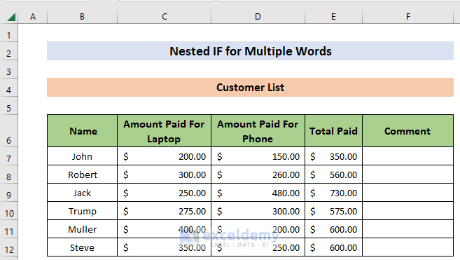
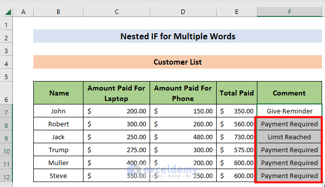
Method 1 – Use of Nested IF Function to Check Multiple Conditions
Steps:
- Use the IF function in the column to get the desired output.
- Type the following formula in the F7 cell:
=IF(E7>=700,"Limit Reached",IF(E7>=500,"Payment Required",IF(E7>300,"Give Reminder","Visit Buyer")))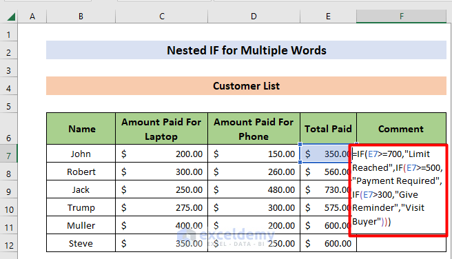
- Hit Enter. This shows the output in cell F7.
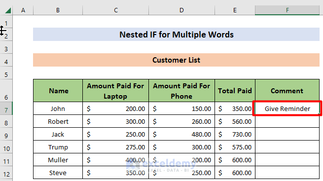
- Hold and drag the AutoFill icon from the bottom right edge of cell F7 to cell F12. This will automatically imply the formula we’ve used in cell F7 and make necessary adjustments to all the cells from F8 to F12.
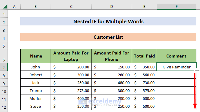
The output in the “Comment” column.
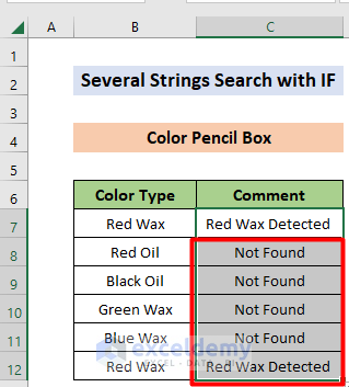
Method 2 – Multiple Strings Search with IF Function
Steps:
- Write the following formula in the C7 cell:
=IF(AND(ISNUMBER(SEARCH("Red",B7)),ISNUMBER(SEARCH("Wax",B7))),"Red Wax Detected ","Not Found")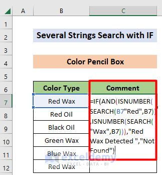
Formula Breakdown
- SEARCH(“Red”,B7) > Here SEARCH function is looking for the position of substring Red in cell B7
Output: 1 - ISNUMBER(1) > ISNUMBER checks whether the argument is a number or not
Output: TRUE - SEARCH(“Wax”,B7) > Here SEARCH function is looking for the position of substring Red in cell B7
Output: 5 - ISNUMBER(5) > ISNUMBER checks whether the argument is a number or not
Output: TRUE - AND(TRUE,TRUE) > AND function has two TRUE arguments.
Output: TRUE - IF(TRUE,”Red Wax Detected “,”Not Found”) > IF will get this type of arguments within it and will return depending on the logic.
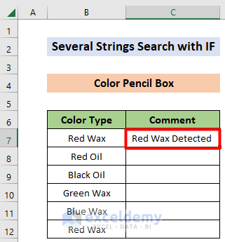
Output: Red Wax Detected
- The output looks like this:
- AutoFill is performed from cell C8 to cell C12
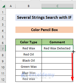
- The dataset is filled with all the desired output.
We wrote an IF statement that contains multiple words in Excel.
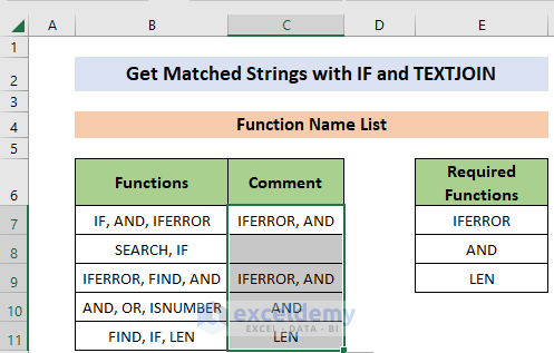
Method 3 – Matching Any String with IF and TEXTJOIN
Steps:
- Type the following formula in the C7 cell and hit Enter.
=TEXTJOIN(", ", TRUE, IF(COUNTIF(B7, "*"&$E$7:$E$9&"*"), $E$7:$E$9, ""))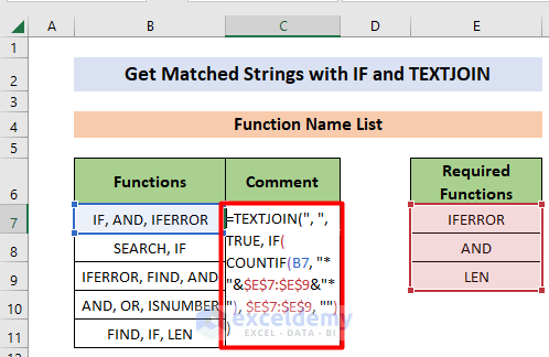
We explained the calculations here (The Active Function is BOLD form and the Output is in BOLD & ITALIC format):
- COUNTIF function returns the number of times a singular entity is present in a predefined range. We’re looking for “IFERROR”, “AND” and “LEN” which span cells E7 to E9. Here Absolute Reference is used to keep this particular part of the formula unchanged in any situation.
- We’re applying the COUNTIF function in cell B7; this is the first argument of the function COUNTIF.
=TEXTJOIN(“, “, TRUE, IF(COUNTIF(B7, “*”&$E$7:$E$9&”*”), $E$7:$E$9, “”))
- The following calculation is shown here:
=TEXTJOIN(“, “, TRUE, IF(COUNTIF($B$7, {“*IFERROR”;”*AND”;”*LEN”}&”*”), $E$7:$E$9, “”))
- Next line:
=TEXTJOIN(“, “, TRUE, IF(COUNTIF($B$7, {“*IFERROR”;”*AND”;”*LEN”}&”*”), $E$7:$E$9, “”))
- The output of the COUNTIF function shows that IFERROR and AND are present in the B7 cell; both one time only, it returned {1:1:0}. Now, the IF function is active.
=TEXTJOIN(“, “, TRUE, IF({1;1;0}, $E$7:$E$9, “”))
- The output of the IF function returns the values “IFERROR” ;“AND”; “ ” as IFERROR and AND are searched in $E$7:$E$9. Now, the TEXTJOIN function is active.
=TEXTJOIN(“, “, TRUE, {“IFERROR”;”AND”;” “})
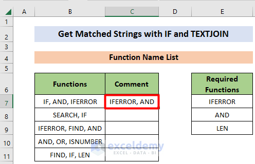
- The task of the TEXTJOIN function is combining the text from multiple ranges and or strings. The output looks like this. And it matches our target.
IFERROR, AND
- See the output in cell C7.
- AutoFill is performed from cell C8 to cell C11
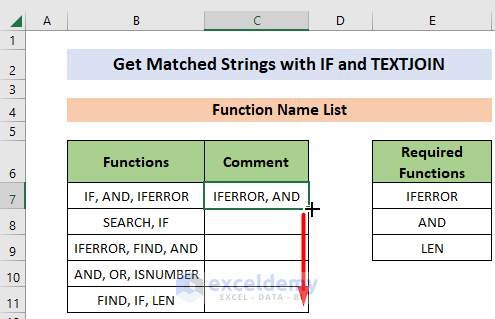
- The dataset is filled with all the desired output.
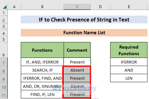
Method 4 – IF to Check Presence of a String in Text
Steps:
- In cell C7, type the following formula and press Enter.
=IF(OR(ISNUMBER(SEARCH("IFERROR",B7)),ISNUMBER(SEARCH("LEN",B7)),ISNUMBER(SEARCH("SUM",B7))),"Present","Absent")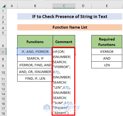
The calculation is shown here (The Active Function is BOLD form and the Output is in BOLD & ITALIC format)
- SEARCH function in bold is being evaluated here. Here SEARCH function is looking for
the position of substring IFERROR in cell B7
=IF(OR(ISNUMBER(SEARCH(“IFERROR”,B7)),ISNUMBER(SEARCH(“LEN”,B7)),ISNUMBER(SEARCH(“SUM”,B7))),”Present”,”Absent”)
- The B7 cell value is passed in the argument of SEARCH function
=IF(OR(ISNUMBER(SEARCH(“IFERROR”,”IF, AND IFERROR”)),ISNUMBER(SEARCH(“LEN”,B7)),ISNUMBER(SEARCH(“SUM”,B7))),”Present”,”Absent”)
- SEARCH function returns the value 10, which is now working as the argument of bold ISNUMBER:
=IF(OR(ISNUMBER(10),ISNUMBER(SEARCH(“LEN”,B7)),ISNUMBER(SEARCH(“SUM”,B7))),”Present”,”Absent”)
- 10 is a number, so, ISNUMBER returns TRUE. At this stage, bolded SEARCH is active, and the abovementioned process is repeated.
=IF(OR(TRUE,ISNUMBER(SEARCH(“LEN”,B7)),ISNUMBER(SEARCH(“SUM”,B7))),”Present”,”Absent”)
- The content of the B7 cell is now in the argument of SEARCH function
=IF(OR(TRUE,ISNUMBER(SEARCH(“LEN”, “IF, AND, IFERROR”)),ISNUMBER(SEARCH(“SUM”,B7))),”Present”,”Absent”)
- SEARCH function returns #VALUE which means “LEN” is not present in B7. Now, the ISNUMBER function is activated.
=IF(OR(TRUE,ISNUMBER(#VALUE!),ISNUMBER(SEARCH(“SUM”,B7))),”Present”,”Absent”)
- ISNUMBER function returns FALSE which means its argument is not a number. Now, the SEARCH function is activated.
=IF(OR(TRUE,FALSE,ISNUMBER(SEARCH(“SUM”,B7))),”Present”,”Absent”)
- Output of the SEARCH function is found, and we got it as explained above.
=IF(OR(TRUE,FALSE,ISNUMBER(SEARCH(“SUM”,“IF, AND, IFERROR”))),”Present”,”Absent”)
- Output of the SEARCH function is also explained above.
=IF(OR(TRUE,FALSE,ISNUMBER(#VALUE!)),”Present”,”Absent”)
- Output of the ISNUMBER function is FALSE and also explained before. Now OR function is active.
=IF(OR(TRUE,FALSE,FALSE),”Present”,”Absent”)
- Output of the OR function is TRUE as at least one argument of the function is TRUE. Now IF function is active.
=IF(TRUE,”Present”,”Absent”)
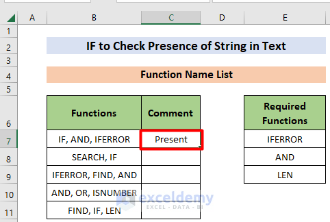
- The output Present. This means the looked-up string(s) are present in cell B7.
Present
- The output is shown in the cell.
- AutoFill is performed from cell C8 to cell C11
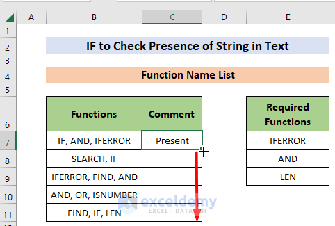
- The dataset is filled with all the desired output.
Download Practice Workbook
You can download the file from the link below.
Related Articles
- Excel IF Statement Between Two Numbers
- How to Find Sum If Cell Color Is Green in Excel
- Use Wildcard with If Statement in Excel
- How to Use Multiple IF Statements in Excel Data Validation


How do i setup a formula to Validate Column K(any value from 0-8;multiple lines (115) and then Display the corresponding value in Words(column T) in Column L.
List in Column S and T
1 Permanent Morning /Day shift
2 Permanent Afternoon shift
3 Permanent Night shift
4 Rotational-Morning and Afternoon Shift
5 Rotational-Morning and Night Shift
6 Rotational-Afternoon and Night Shift
7 Rotational-Morning ,Afternoon and Night Shift
8 Employees who work different workschedules on the same Org unit
If this make sense? tx
Dear Danny Van Straten,
If you need any types of customized templates you may contact us through [email protected]
We have a expert team to create any types of professional templates.
Regards
ExcelDemy