The ISNUMBER function in Microsoft Excel is commonly used to determine whether a given argument contains a numerical value.
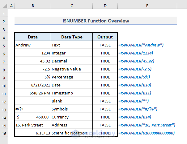
The above screenshot is an overview of the tutorial, representing a few applications of the ISNUMBER function in Excel.
Introduction to the ISNUMBER Function
- Function Objective
The ISNUMBER function serves to check whether a value is numeric or not.
- Syntax
=ISNUMBER(value)
- Argument Explanation
| Argument | Required/Optional | Explanation |
|---|---|---|
| value | Required | The value you want to evaluate. |
- Return Parameter
A boolean value: TRUE if the value is numeric, and FALSE otherwise.
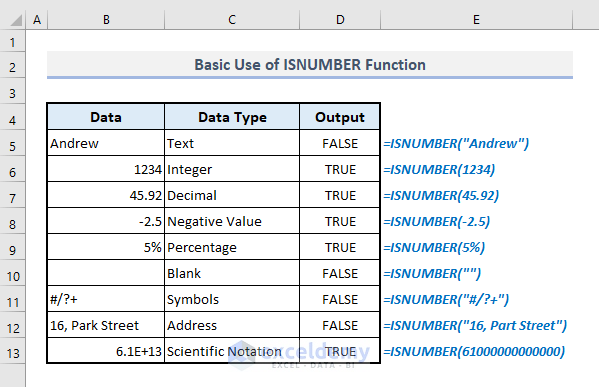
Method 1 – Basic Use of Excel ISNUMBER Function
Consider the data in Column B shown in the screenshot below. In Column D, the outputs indicate whether the selected data are numbers or not, represented by boolean values: TRUE and FALSE, respectively. Since the ISNUMBER function accepts a value as its argument, the formula in the first output cell (D5) is as follows:
=ISNUMBER("Andrew")The function returns FALSE because Andrew is a text, not a numeric value. You can apply the same approach to other values in Column B, with the corresponding formulas displayed in Column D.
Method 2 – Using ISNUMBER with Cell References in Excel
The ISNUMBER function also accepts cell references or ranges as arguments. Let’s explore how it works with the cell references from all the data in Column B. For example, in output cell D5, the formula with the ISNUMBER function and the cell reference (B5) for the name Andrew is:
=ISNUMBER(B5)After pressing Enter, you’ll obtain a similar result as in the previous section. You can extract other outputs in Column D using cell references from Column B in the same manner.

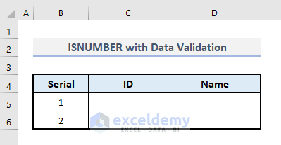
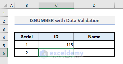
Method 3 – Applying ISNUMBER for Data Validation
Let’s use the ISNUMBER function for data validation. In the table below, Column C will only contain numerical values for ID numbers. If someone attempts to input a text value or a letter, an error message will appear. Here’s how to set up these parameters:
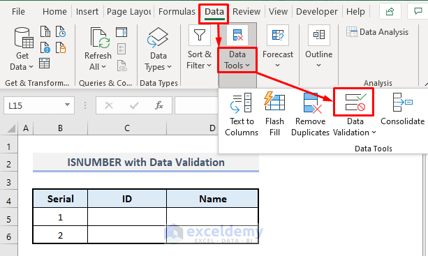
Step 1
- From the Data ribbon, select the Data Validation command from the Data Tools drop-down.
- A dialogue box named Data Validation will open.
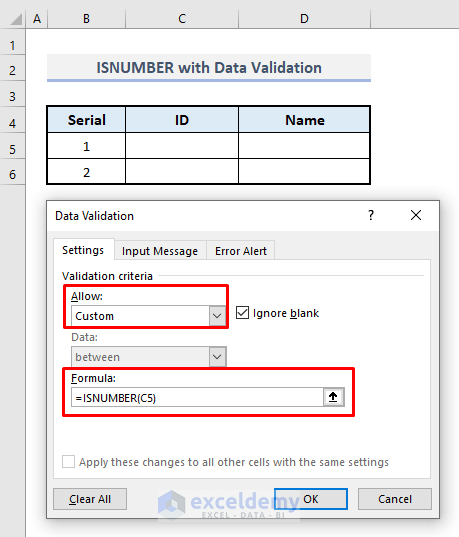
Step 2
- Choose Custom from the Allow list as the validation criteria.
- In the formula box, enter:
=ISNUMBER(B5)
- Go to the Error Alert tab.
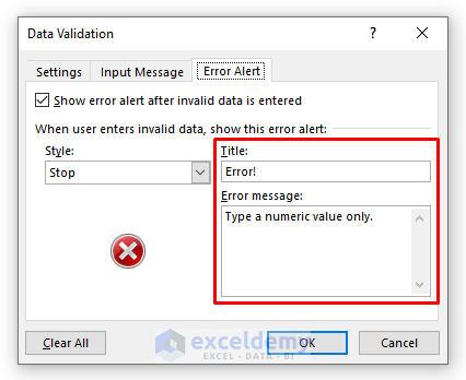
Step 3
- Enter Error! in the Title box.
- Set the Error message to Type a numeric value only.
- Press OK to finalize the input criteria settings.
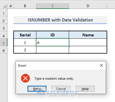
Step 4
- Try inputting a letter or an alpha in Cell C5; a message box will appear.
- The message box displays the title and error message defined in the Data Validation dialogue box.
- Press Cancel to dismiss the message box.
Step 5
- Input a numerical value (e.g., 115) in Cell C5.
- No message box appears because the cell is defined for numerical input only.
Read More: How to Use COUNTIF & ISNUMBER to Count Numbers in Excel
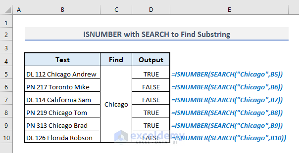
Method 4 – Combining ISNUMBER and SEARCH Functions to Find a Substring
Consider the table below, where Column B contains various text data. Our goal is to identify which cells in that column contain the specific word Chicago. We can achieve this by combining the ISNUMBER function with the SEARCH function. For the first text value in Cell B5, the required formula to find the word Chicago is:
=ISNUMBER(SEARCH("Chicago",B5))- Press Enter, and the formula will return the boolean value TRUE.
- Drag the formula down to the rest of Column D by using Fill Handle to fill.
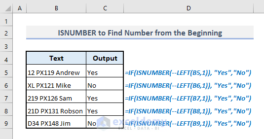
Method 5 – Identifying Texts That Start with a Number Using ISNUMBER, LEFT, and IF Functions
The LEFT function extracts a specified number of characters from text data. By combining the ISNUMBER, LEFT, and IF functions, we can easily determine whether a text starts with a numerical value or not.
Consider the dataset below, where the output cells in Column C will return Yes if the criteria are met (i.e., the text starts with a number), otherwise they will return No.
Formula for the First Text Value:
=IF(ISNUMBER(--LEFT(B5,1)), "Yes","No")- Press Enter and autofill the entire Column C to obtain all other outputs at once.
How Does the Formula Work?
- The LEFT function extracts only the first character of the text.
- The use of double-unary (–) converts the text data into numerical values.
- The ISNUMBER function identifies whether the extracted value is numeric (returns TRUE) or not (returns FALSE).
- Finally, the IF function combines the output of the ISNUMBER function to return Yes or No based on the boolean values.
Read More: Use ISNUMBER Function with IF and Then Statements in Excel
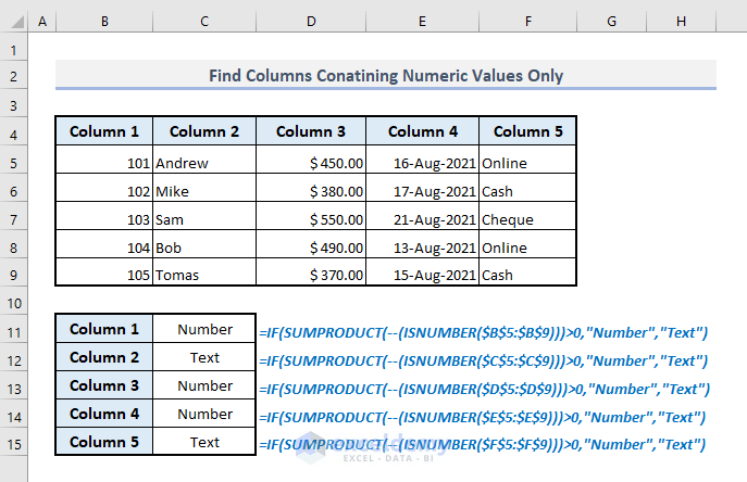
Method 6 – Determining Data Types Using ISNUMBER and SUMPRODUCT
In the below table, there are random columns with specific data types. By combining the ISNUMBER and SUMPRODUCT functions, we can find out the data types for all available columns.
For the first column (Column 1 in the header row), the formula in Cell C11 to find the data type should be:
=IF(SUMPRODUCT(--(ISNUMBER($B$5:$B$9)))>0,"Number","Text")- Press Enter, and the formula will return Number. You can use a similar procedure to determine data types for other columns.
How Does the Formula Work?
- The ISNUMBER function returns boolean values (TRUE or FALSE) for all data in the selected column.
- The double-unary (–) converts each boolean value: TRUE to 1 and FALSE to 0.
- The SUMPRODUCT function adds up the numerical values obtained in the previous step.
- The IF function evaluates whether the sum from the preceding step is greater than zero (0) and returns Number or Text accordingly.
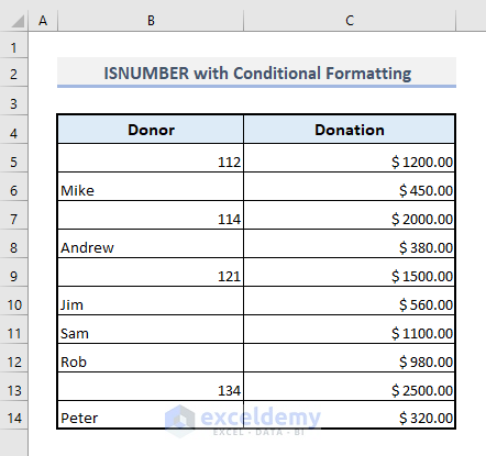
Method 7 – Using ISNUMBER with Conditional Formatting in Excel
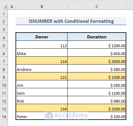
In this method, we’ll explore how to use the ISNUMBER function in Conditional Formatting to highlight cells or rows in a table based on specific criteria. Consider the following dataset, where Column B contains donor names and IDs. We want to highlight rows for donors whose ID numbers are visible in Column B and who have donated $1500 or more.
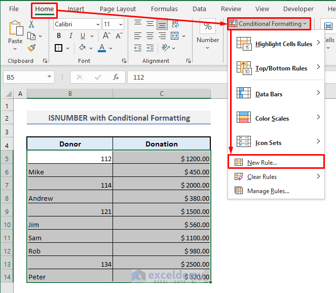
Step 1
- Select the range of cells B5:C14.
- Under the Home tab, choose New Rule from the Conditional Formatting drop-down.
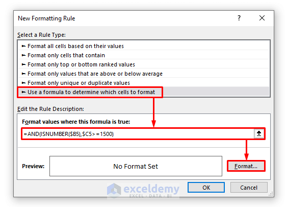
Step 2
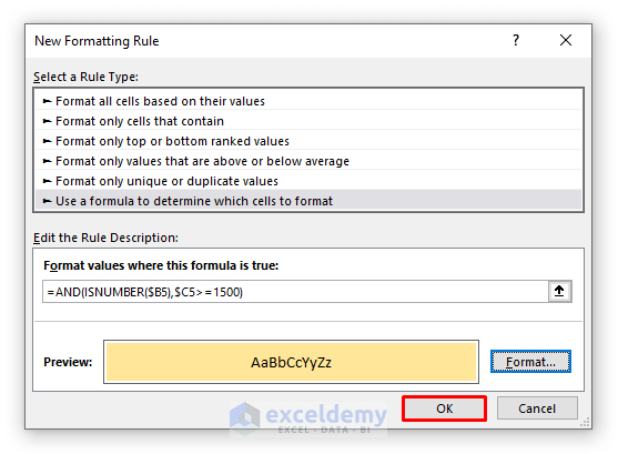
- Select the rule type: Use a formula to determine which cells to format.
- In the formula box, enter:
=AND(ISNUMBER($B5),$C5>=1500)- Click on the Format option.
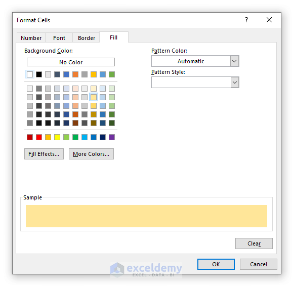
Step 3
- Choose a color to highlight the rows.
- Press OK to apply the formatting.
Step 4
- A preview will be shown at the bottom bar of the New Formatting Rule dialogue box.
- Press OK.
The result can be seen below:
Read More: [Fixed] Excel ISNUMBER Not Working
Things to Keep in Mind
Here are the key points to keep in mind regarding the ISNUMBER function in Excel:
- Argument Types:
- While the ISNUMBER function typically takes a value or a cell reference as its argument, you can also input a formula to determine if the resulting value is numeric or not.
- Dates and Times:
- In Excel, dates and times are also considered numeric values. Therefore, the ISNUMBER function will return TRUE for dates and times within strings.
- Function Group:
- The ISNUMBER function belongs to the group of IS functions, which are used for logical tests.
- Error Handling:
- The function does not return any error; it simply examines whether the given input is numerical or not.
- Input Restrictions:
- You cannot directly input a date or time into the argument of the ISNUMBER function. If you do, the function will return FALSE. Instead, use the DATE and TIME functions to input dates or times for the ISNUMBER argument.
Download Practice Workbook
You can download the practice workbook from here:
<< Go Back to Excel Functions | Learn Excel
Get FREE Advanced Excel Exercises with Solutions!
