Method 1 – Basic Use of LEFT Function: Extract String from Left Side
Steps:
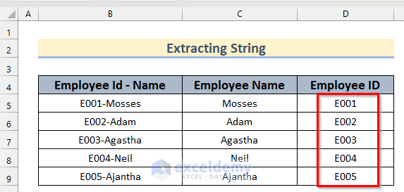
- Select Cell D5 and insert the following formula.
=LEFT(B5,4)- Press Enter and drag down the Fill Handle tool to autofill this formula for the rest of the cells.
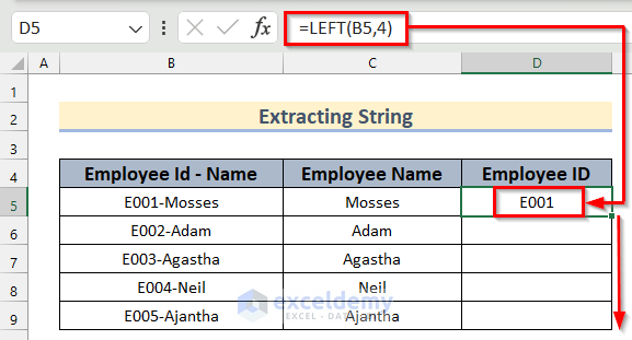
In the formula, we inserted cell B4 as text and 4 as num_chars.
- Tthe LEFT function will provide the Employee ID for all the values.
Method 2 – Insert Excel LEFT & SEARCH Functions to Extract Text up to Specific Character
Steps:
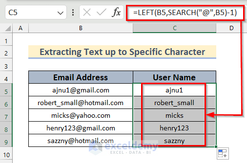
- Insert the following formula in cell C5.
=LEFT(B5,SEARCH("@",B5)-1)- Press Enter.
- Drag-down the Fill Handle tool to use this formula for the rest of the Cells.
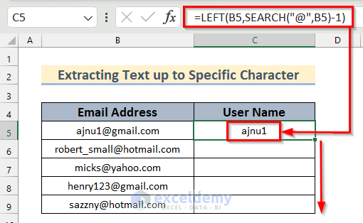
We searched for @, the SEARCH function would return the position of @. We wanted up to @, so we subtracted 1 from the position number. This provided the user name.
- The LEFT and SEARCH functions will provide the User Name for all the values.
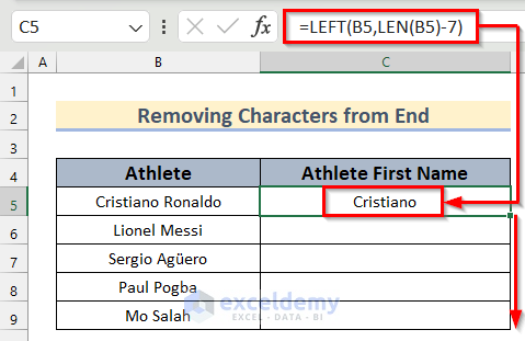
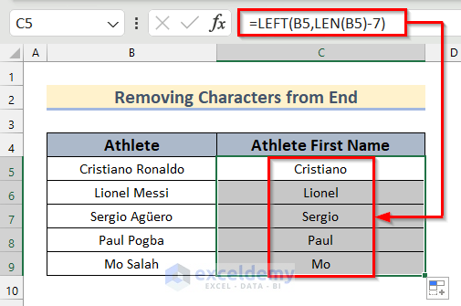
Method 3 – Remove Characters from End of a String Using LEFT & LEN Functions
Steps:
- Select cell C5 and insert the following formula.
=LEFT(B5,LEN(B5)-7)- Press Enter and drag down the Fill Handle tool to autofill this formula for the rest of the cells.
How Does the Formula Work?
- The LEN function determines the total number of characters of the given string.
- The LEFT formula removes the unwanted part of the string.
- Yhe LEFT function returns the rest of the characters in Excel.
- You will get the Athlete’s First Name using the LEFT and LEN functions.
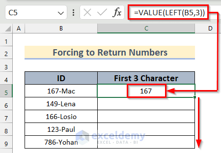
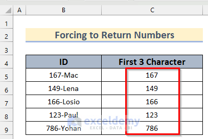
Method 4 – Force to Return Numbers Applying Excel LEFT & VALUE Functions
Steps:
- Select Cell C5 and type the following formula.
=VALUE(LEFT(B5,3))- Press Enter and drag down the Fill Handle tool.
How Does the Formula Work?
- Initially, The LEFT function returns the first 3 characters from the ID.
- The VALUE function converts text that appears in a recognized format into a numeric value.
- Using the formula, we have found the 3 characters from the string and converted them into numeric.
Things to Remember
- If we provide a value less than 0 into the num_chars field, then it will provide #VALUE! Error.
- Secondly, for dates, you may not find the exact value you are wanting. From a date, if you want to find the day portion, you may write LEFT with 2 in the num_chars field. But will find another value, not the day value of the provided date.
- Usually, Excel stores dates as sequential serial numbers. 1 January 1900 is the 1st date, and its serial number is 1. From there every date has its subsequent serial number. Thus, the functions convert dates to their respective serial number before doing the operations.
- Therefore, if you set the cell containing the date into General you will find the serial number. The formula will extract from that serial number.
- Finally, you can also provide the text value directly into the function.
Download Practice Workbook
You are welcome to download the practice workbook from the link below.
<< Go Back to Excel Functions | Learn Excel
Get FREE Advanced Excel Exercises with Solutions!
