Overview of the Excel ROW Function
- Description
The ROW function returns the row number for a given reference. The reference may be a cell or cell range. If the reference is not specified (as the argument is optional), the ROW function automatically considers the cell containing the formula as a reference.
- Generic Syntax
=ROW (reference)- Argument Description
| ARGUMENT | REQUIREMENT | EXPLANATION |
|---|---|---|
| reference | Optional | A reference to a cell or range of cells |
- Returns
The row number of the reference cell(s)
Example 1 – Basic Examples Using the ROW Function
Steps:
- In the example below, we have used the ROW function without any argument in cell D6.
=ROW()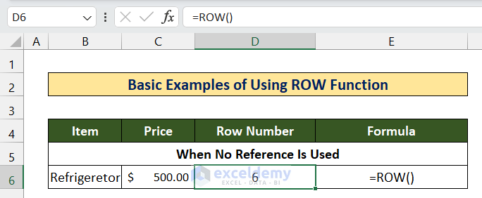
- It took D6 as its argument by default and returned the row number of D6.
- We will see the application of the ROW function while giving a single cell as an argument.
- In D8 and D9, enter the following two formulas:
=ROW(B8)=ROW(B9)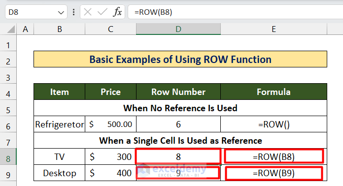
- As a result, we get their row numbers (8 and 9).
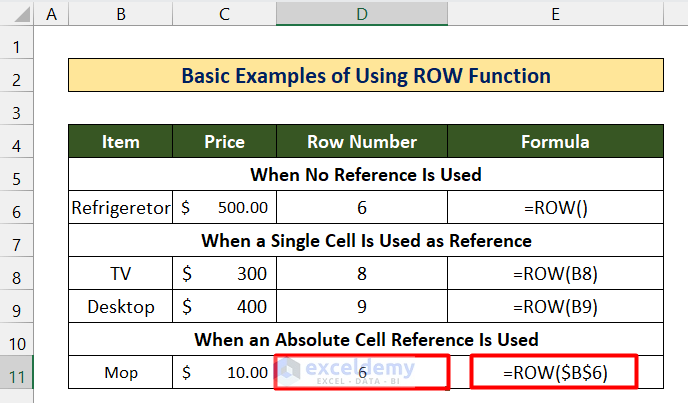
- We will see the application when we use an Absolute Cell reference ($B$6) as an argument.
- In D11, enter the following formula:
=ROW($B$6)- The result is the same: the row number of B6 is 6.
- We will see the case when we use multiple cells/ranges of a single row as an argument.
- In cell D13, enter the following formula:
=ROW(B13:C13)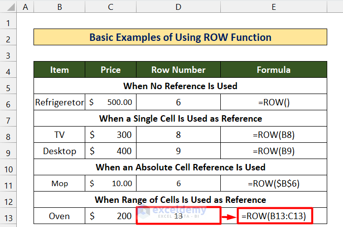
- We get the expected row number, which is 13.
Example 2 – Creating Dynamic Arrays Utilizing the ROW Function
Steps:
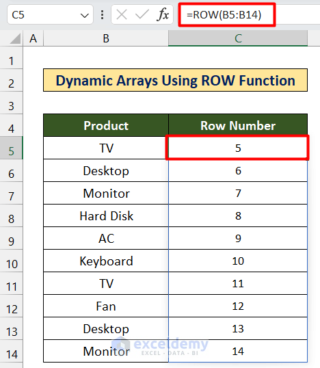
- If you are a Microsoft 365 subscriber and use the ROW function for the range of cells in a column (like B5:B14 in the following figure), you’ll get not a single row number.
- You’ll get a range of dynamic arrays. Microsoft recommends this feature for convenience in the calculation process rather than using regular arrays.
- The formula is:
=ROW(B5:B14)- You will get the row number from 5 to 14 in a column as a dynamic array like this figure below.
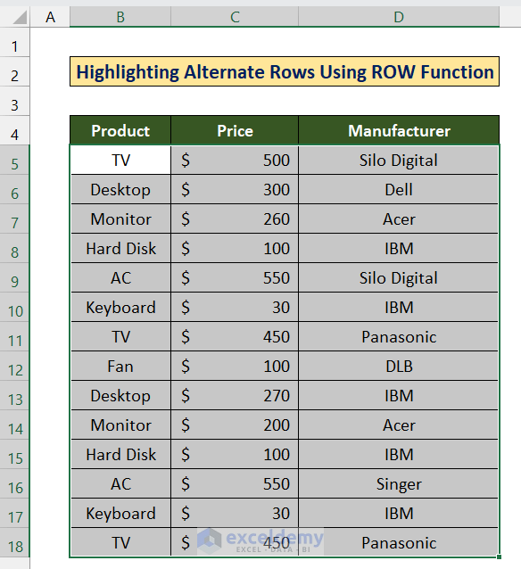
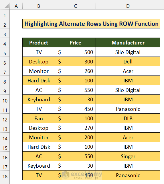
Example 3 – Highlighting Alternate Rows Applying the ROW Function
Steps:
- Select the data.
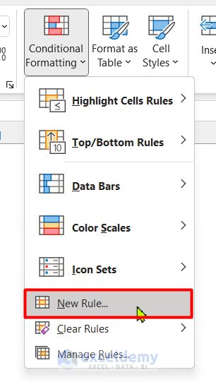
- Go to the Conditional Formatting toolbar from the Styles command bar and choose New Rule.
- Click to Use a new formula to determine which cells to format.
- In the formula bar, enter the following formula and click OK.
=MOD(ROW(),2)=0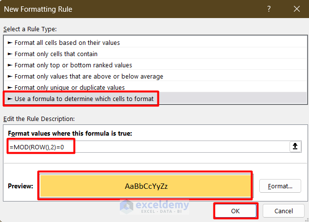
- You will see that the even row numbered(6,8,10, etc.) cells have been formatted.
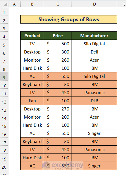
Method 4 – Using the ROW Function to Show Groups of Rows
Steps:
- Select the cells and follow the steps shown in example 3 to go to Conditional Formatting.
- Enter the following equation in the formula bar:
=MOD(INT((ROW()-1)/4)+1,2)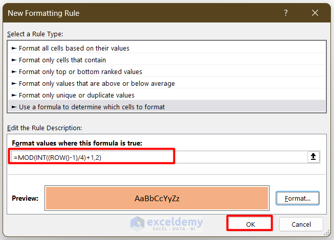
- The result will be like this below.
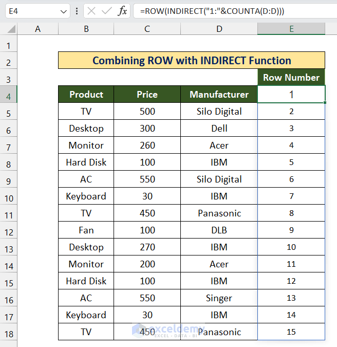
Method 5 – Combining ROW with the INDIRECT Function
Steps:
- In cell E4, enter the following formula:
=ROW(INDIRECT("1:"&COUNTA(D:D)))- Click Enter. You will see a result like this.
Method 6 – Use ROW with the INDEX MATCH Formula
Let’s imagine you have a dataset of products with the manufacturer, price, etc. Now, you want to find the row number for a specific product. (see the figure below)
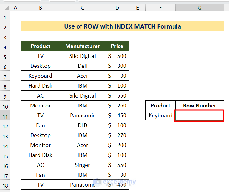
Steps:
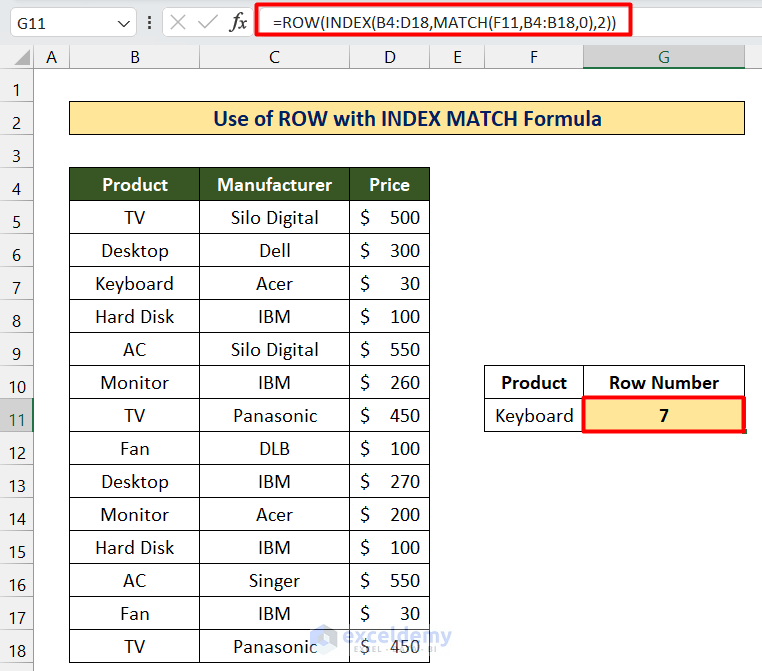
- In the G11, enter the following formula:
=ROW(INDEX(B4:D18,MATCH(F11,B4:B18,0),2))- Press Enter. You will have a result like this.
Method 7 – Utilizing a Combination of ROW and HLOOKUP Functions
The HLOOKUP function looks up data from a cell range like VLOOKUP, but it asks for the row number. To acquire the desired data using HLOOKUP, please input the row number.
=HLOOKUP(H8,C4:E18,ROW(E8),0)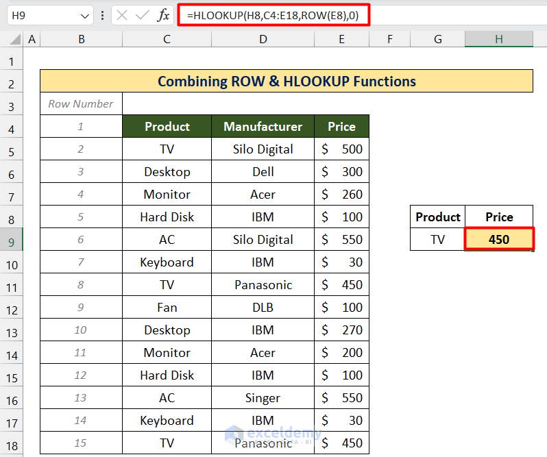
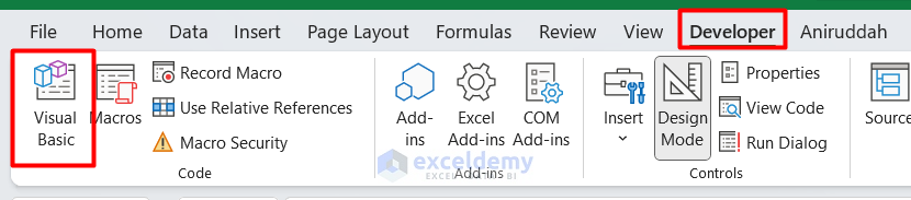
Method 8 – Getting a Row Number By Using VBA in Excel
Steps:
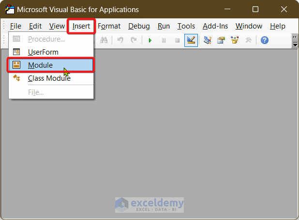
- Click on the Developer tab and select Visual Basic to open the VB window. Alternatively, you can also click Alt + F11.
- In the VB window, click on Insert > Module.
- A new module will open. Paste the following VBA code into your module:
Sub Excel_ROW_Function()
'declare a variable
Dim ws As Worksheet
Set ws = Worksheets("8.VBA ROW")
'apply the Excel ROW function
ws.Range("D5") = ws.Range("B5").Row
ws.Range("D6") = ws.Range("B6").Row
ws.Range("D7") = ws.Range("B7").Row
ws.Range("D8") = ws.Range("B8:C8").Row
End Sub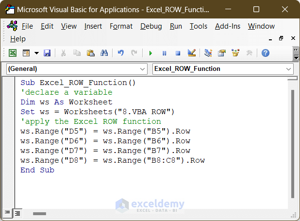
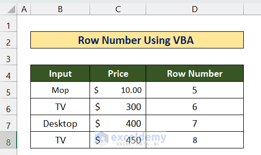
- Run the code to see the row numbers appear in the Row Number column.
What Are the Common Errors While Using the ROW Function?
| Common Errors | When they show |
|---|---|
| #N/A | Occurs when the required value is not found. |
Things to Remember
- While using conditional formatting, be careful when selecting cells where the formatting will be applied.
- Use VBA code only when you have a large data set.
Download the Practice Workbook
Download this workbook to practice.
<< Go Back to Excel Functions | Learn Excel
Get FREE Advanced Excel Exercises with Solutions!
