In Microsoft Excel, HLOOKUP or Horizontal Lookup function is generally used to extract data from a table or an array based on searching for a specified value in the topmost row and the corresponding column.

The above screenshot is an overview of this article, representing an application of the HLOOKUP function in Excel. We’ll use this dataset to illustrate our methods.
Introduction to the HLOOKUP Function
- Function Objective:
HLOOKUP function searches for a value in the top row of a table or array of values and returns the value in the same column from the specified row.
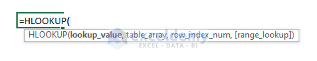
- Syntax:
=HLOOKUP(lookup_value, table_array, row_index_num, [range_lookup])
- Arguments Explanation:
| Argument | Compulsory/Optional | Explanation |
|---|---|---|
| lookup_value | Compulsory | The value to be looked for in the table. |
| table_array | Compulsory | The table or an array of cells where the specified value will be looked for. |
| row_index_num | Compulsory | Position of the row in the table from where the data will be extracted based on the column containing the lookup value. |
| [range_lookup] | Optional | Lookup criteria. TRUE for Approximate Match and FALSE for Exact Match. |
How to Use HLOOKUP Function in Excel: 8 Suitable Approaches
Example 1 – Finding an Exact Match
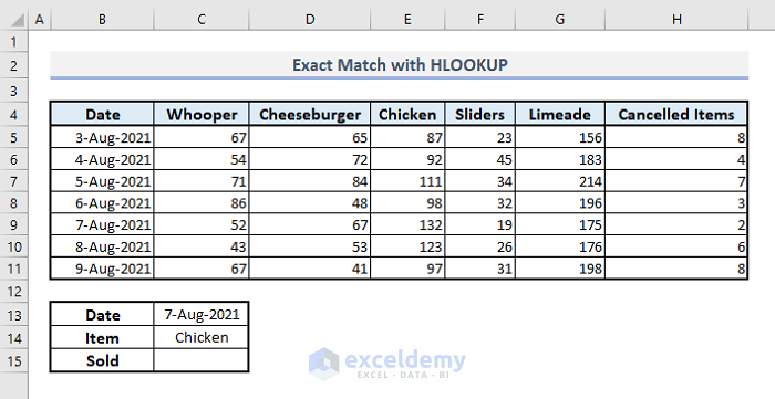
The table below represents the number of orders of some foods on some consecutive dates. Column H shows the number of canceled items or orders on those dates. By using the HLOOKUP function, we’ll find out how many fried chickens were sold on 7 August 2021.
Steps:
- In cell C15, enter the following formula:
=HLOOKUP(C14,B4:H11,6,FALSE)- Press Enter.
The function returns 132. So, a total of 132 pieces of fried chickens was sold on the specified date.
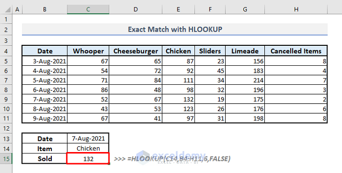
In the 4th argument of the HLOOKUP function, we defined the range_lookup as FALSE, meaning function will search for an exact match of the lookup item ‘Chicken’ in the table.
Example 2 – Approximate Match
We can use Approximate Match by setting the 4th argument of the HLOOKUP function as TRUE. If our search criterion coincides partially with the exact name we’re looking for, then the function will consider that a match, and return it in the output cell.
Let’s replace the name of the food item ‘Chicken’ with ‘Kitchen’ to see if our function works accordingly, as ‘Chicken’ and ‘Kitchen’ sound almost similar.
Steps:
- In cell C15, enter the following formula:
=HLOOKUP(C14,B4:H11,6,TRUE)- Press Enter.
The resultant value of 132 is returned.
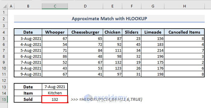
So, by using TRUE in the 4th argument, the proper match was returned even after we typed the name of an item that is absent from the table. In cell C14, input some other different or partially matched names present in the table and see what the function returns.
Example 3 – Using HLOOKUP with MATCH Function
In order not to have to define the row number every time inside the HLOOKUP function, but rather change the date or value in cell C13 and find the result, we can use the MATCH function to define the row number of the data present in the corresponding cell.
For example, cells C13 and C14 show the date and the food item respectively. Let’s find out how many sliders were sold on that specified date in cell C13.
Steps:
- In cell C15, enter the following formula:
=HLOOKUP(C14,B4:H11,MATCH(C13,B4:B11,0),FALSE)- Press Enter to return the result.
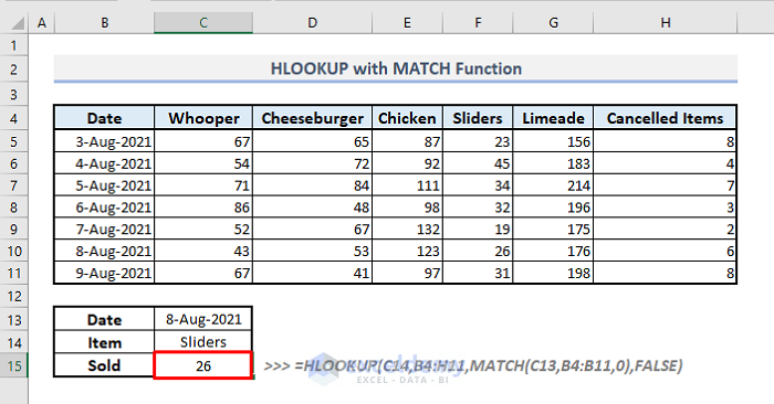
Now, every time we modify the date and name of the food item in cells C13 and C14, the output will update accordingly in cell C15.
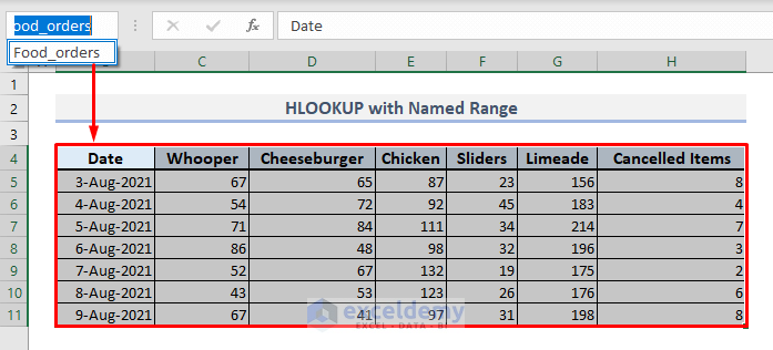
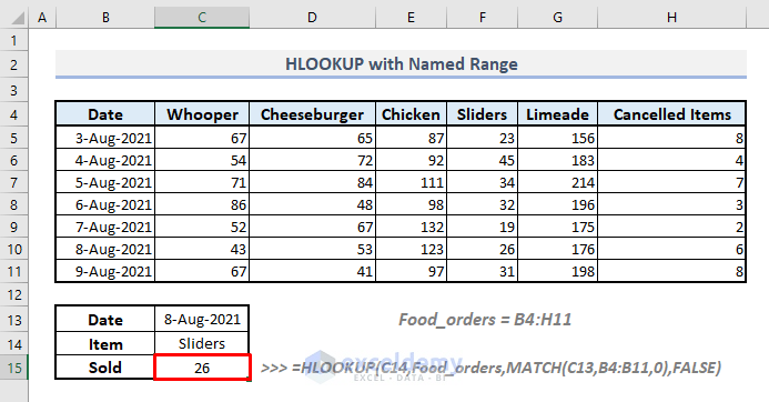
Example 4 – Defining Named Range for Table Array inside the HLOOKUP Function
By defining the name of the table, we can replace the range of cells or array with the named range in the 2nd argument of the HLOOKUP function.
Steps:
- Select the entire table and go to the Name Box on the left top.
- Edit the name, for example to Food_orders.
- Select the output cell C15 where we’ll extract the number of sliders sold on 8 August 2021 and enter:
=HLOOKUP(C14,Food_orders,MATCH(C13,B4:B11,0),FALSE)- Press Enter to return the result.
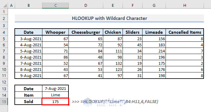
Example 5 – Inserting Wildcard for Approximate Match
By using the wildcard character Asterisk(*) before and/or after a text, we can look for the string containing that text inside. It’s an alternative to the Approximate Match discussed above but much more precise.
Suppose we want to find out the number of orders for a food item containing the text ‘Lime’ on 7 August, 2021.
Steps:
- In cell C15, enter the following formula:
=HLOOKUP("*Lime*",B4:H11,6,FALSE)- Press Enter to return the result.
Example 6 – Cell Reference from Another Worksheet
We can use the HLOOKUP function to extract data from other Excel worksheets too. For example, suppose we have a table like the picture below in Sheet1.
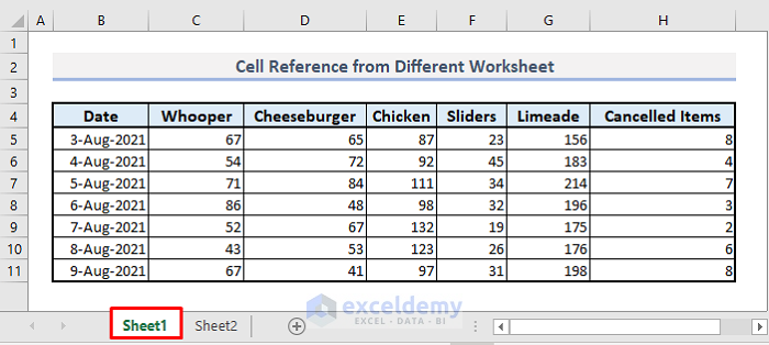
In Sheet 2, we’ll extract the data from Sheet1. Let’s find out the number of orders of the food item Sliders on 6 August 2021.
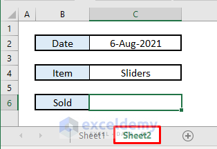
Steps:
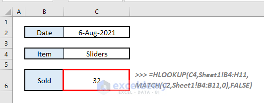
- In cell C6 in Sheet2 enter the following formula:
=HLOOKUP(C4,Sheet1!B4:H11,MATCH(C2,Sheet1!B4:B11,0),FALSE)- Press Enter.
The function returns the value 32 in Sheet1.
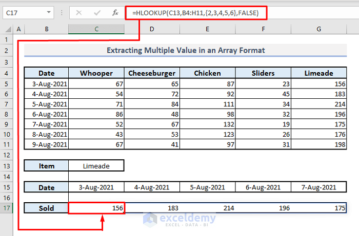
Example 7 – Extracting Multiple Values
By inserting an array containing the row numbers of the table inside the HLOOKUP function, we can pull out multiple data based on specific criteria.
For example, let’s find the number of the food item Limeade sold on 5 successive days beginning on 3 August, 2021.
Steps:
- In cell C17, enter the following formula:
=HLOOKUP(C13,B4:H11,{2,3,4,5,6},FALSE)- Press Enter,
The resultant values will be returned as an array in a row.
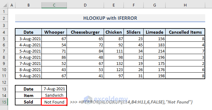
Example 8 – Using IFERROR with HLOOKUP to Modify Error Message If Found
When the HLOOKUP function can’t find a defined lookup value in the table, it’ll return a Value Not Available (#N/A) error. We can modify this error message to “Not Found” by using the IFERROR function.
IFERROR function returns value_if_error if the expression is an error and the value of the expression itself otherwise. The generic formula of this function is:
=IFERROR(value, value_if_error)
In our dataset, let’s now find out the number of sandwiches sold on 7 August 2021. If the item is absent in the table, the function will return a “Not Found” message.
Steps:
- In cell C15, enter the following formula:
=IFERROR(HLOOKUP(C14,B4:H11,6,FALSE),"Not Found")- Press Enter to return the result based on the lookup criteria and defined message.
Things to Keep in Mind
HLOOKUP function only looks for the data based on the selected row(s). To extract data from selected column(s), use the VLOOKUP function.
HLOOKUP function searches for the value in the first row. If your data is present in another row, rearrange the table to keep the criteria in the first row.
HLOOKUP function is not case-sensitive, so it will consider ALEX and alex identical.
The 4th argument (range_lookup) of the HLOOKUP function is optional. Unless otherwise specified, the default value is TRUE, which represents Approximate Match.
Download Practice Workbook
<< Go Back to Excel Functions | Learn Excel
Get FREE Advanced Excel Exercises with Solutions!
