1. Method 1 – Use of COUNTIF Function with Comparison Operator in Excel
Use a comparison operator inside the COUNTIF function to show how many participants have scored more than 70 in the contest.
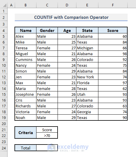
Steps:
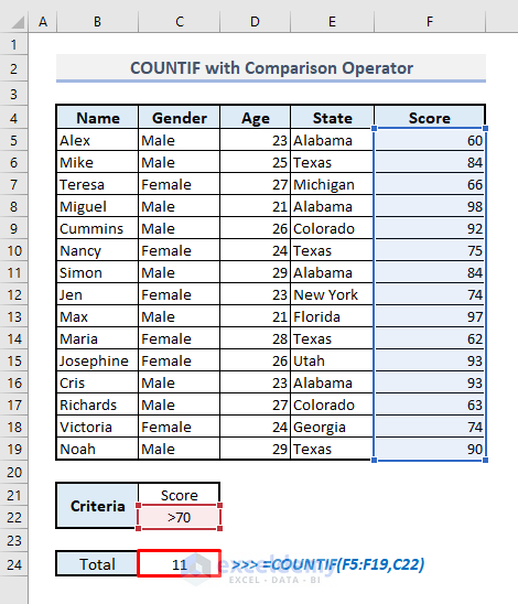
➤ Select the output cell C24 and type:
=COUNTIF(F5:F19,C22)Or,
=COUNTIF(F5:F19,">70")➤ Press Enter, and you’ll see the number of participants who have scored more than 70 in the contest.
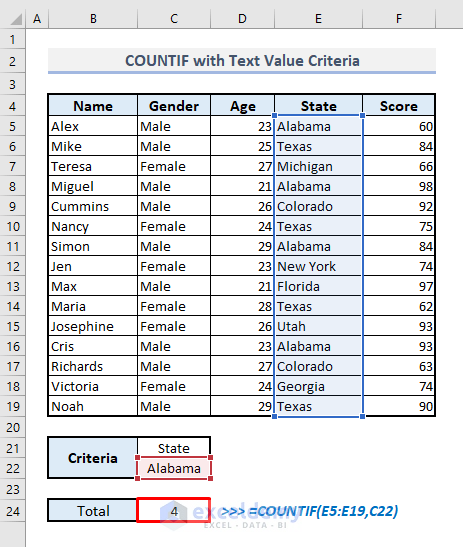
Method 2 – Using COUNTIF Function with Text Criteria in Excel
Steps:
➤ In the output cell C24, the related formula will be:
=COUNTIF(E5:E19,C22)Or,
=COUNTIF(E5:E19,"Alabama")➤ Press Enter and the function will return 4; a total of 4 participants are from Alabama state.
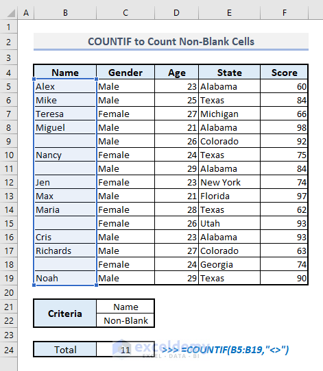
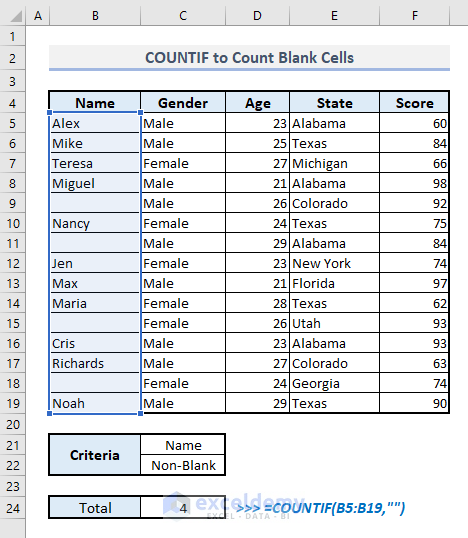
Method 3 – COUNTIF Function to Count Blank or Non-Blank Cells
Steps:
➤ The required formula in the output cell C24 will be:
=COUNTIF(B5:B19,"<>")➤ After pressing Enter, you’ll be displayed the resultant value immediately.
Count the blank cells in column B, then the required formula in cell C24 will be:
=COUNTIF(B5:B19,"")Press Enter to find the total number of blank cells in the output cell.
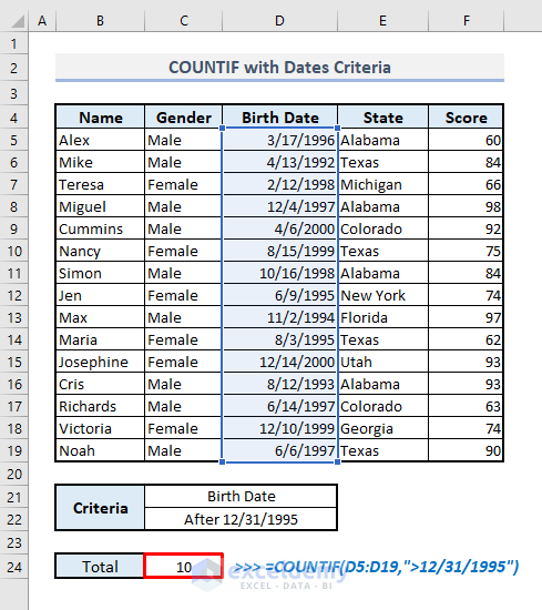
Method 4 – Including Dates Criteria inside the COUNTIF Function in Excel
Steps:
➤ Select cell C24 and type:
=COUNTIF(D5:D19,">12/31/1995")➤ Press Enter; the resultant value will be 10.
The date format in the criteria argument has to be MM/DD/YYYY.
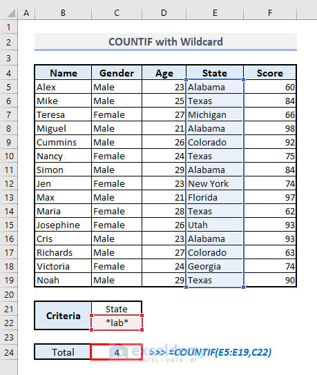
Method 5 – Application of Wildcards inside the COUNTIF Function for Partial Match Criteria
Steps:
➤ In the output cell C22, the related formula for the partial match should be:
=COUNTIF(E5:E19,C22)Or,
=COUNTIF(E5:E19,"*lab*")➤ Press Enter, and you’ll find the total number of participants from the state of Alabama, as it contains the defined text ‘lab’ in its name.
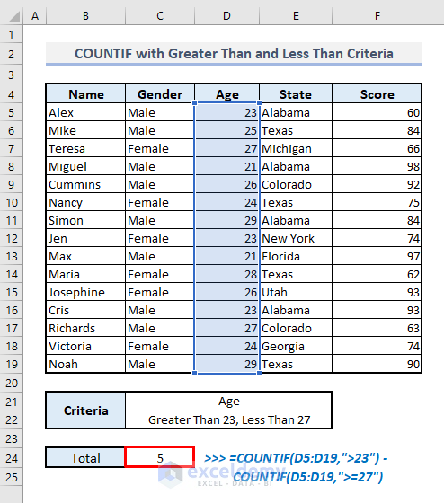
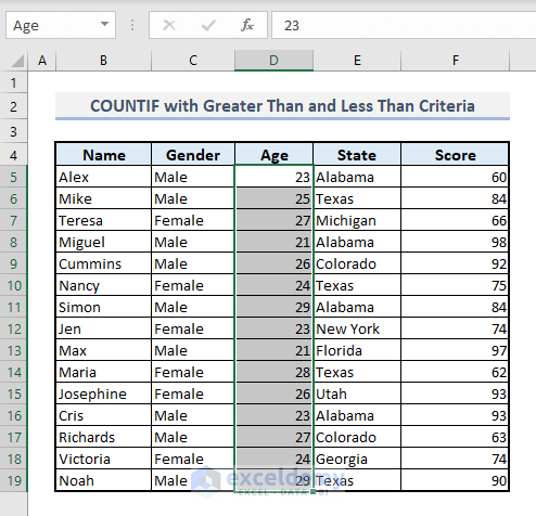
Method 6 – COUNTIF Function for Values Greater Than and Less Than Criteria
Steps:
➤ Select the output cell C24 and you have to type:
=COUNTIF(D5:D19,">23")-COUNTIF(D5:D19,">=27")➤ After pressing Enter, you’ll get the total number of participants aged between 23 and 27 years.
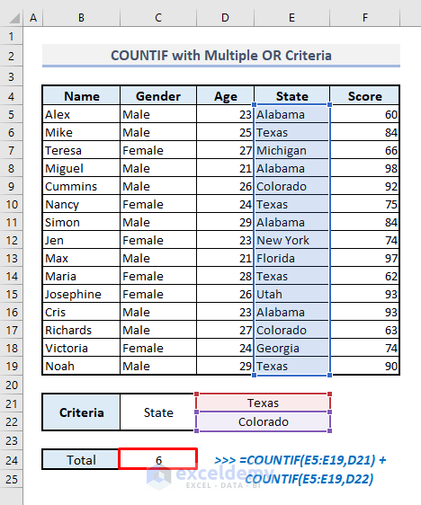
Method 7 – Use of COUNTIF with Multiple OR Criteria in Excel
Steps:
➤ In the output cell C24, the required formula will be:
=COUNTIF(E5:E19,D21)+COUNTIF(E5:E19,D22)Or,
=COUNTIF(E5:E19,"Texas")+COUNTIF(E5:E19,"Colorado")➤ Press Enter, and you’ll see the resultant value at once.
Method 8 – Using COUNTIF to Find Duplicates in Two Columns
Steps:
➤ Select the output cell B22 and type:
=SUMPRODUCT(--(COUNTIF(B5:B19,C5:C19)>=1))➤ Press Enter; you’ll see a total of 4 names that are present in both columns.
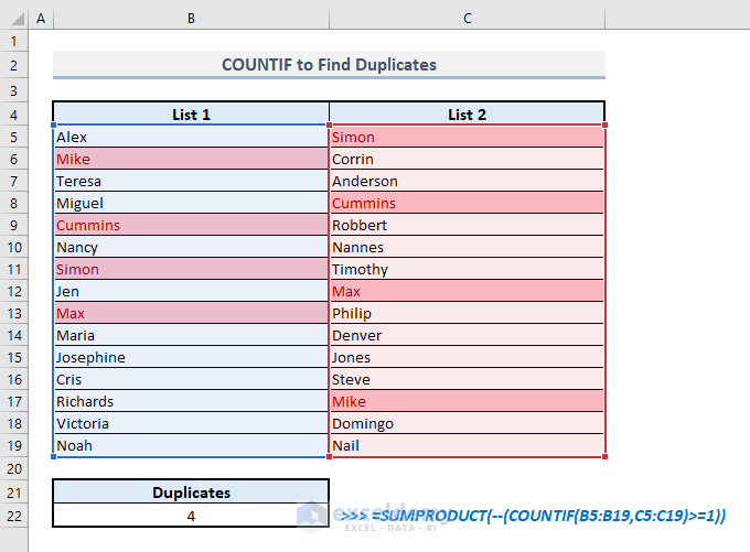
How Does This Formula Work?
➤ Here COUNTIF function extracts the total number of matches for each name in an array and returns:
{1;0;0;1;0;0;0;1;0;0;0;0;1;0;0}
➤ With the comparison operator, the resultant values convert the numbers equal to or more than 1 into a logical value- TRUE, and for 0, it returns FALSE. So, the overall return values look like then:
{TRUE;FALSE;FALSE;TRUE;FALSE;FALSE;FALSE;TRUE;FALSE;FALSE;FALSE;FALSE;TRUE;FALSE;FALSE}
➤ The Double-Unary(–) used before the COUNTIF function converts all of these booleans into numerical values- 1(TRUE) and 0(FALSE). The function will return:
{1;0;0;1;0;0;0;1;0;0;0;0;1;0;0}
➤ The SUMPRODUCT function sums all these numerical values and returns 4.
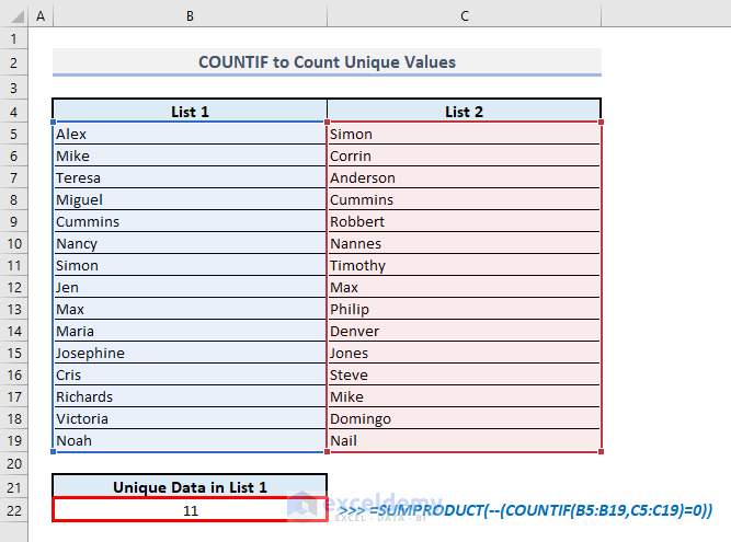
Method 9 – Use of COUNTIF to Extract Unique Values from Two Columns in Excel
Steps:
➤ The related formula in the output cell B22 to find the number of unique values from two different columns will be:
=SUMPRODUCT(--(COUNTIF(B5:B19,C5:C19)=0))➤ After pressing Enter; the desired output right away.
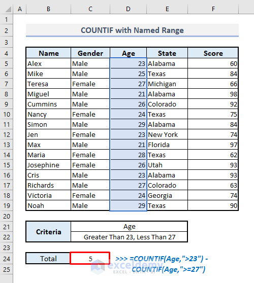
Method 10 – Inserting Named Range in the COUNTIF Function to Count Cell with Criteria
By using this named range- Age, we’ll find out the total number of participants aged between 23 and 27 years.
Steps:
➤ Select the output cell C24 and type:
=COUNTIF(Age,">23") - COUNTIF(Age,">=27")➤ Press Enter; the formula will return 5.
Things to Keep in Mind
You cannot input more than one criterion in the COUNTIF function. You have to use the COUNTIFS function for the inputs of multiple criteria.
COUNTIF function is not case-sensitive. If you need to count case-sensitive cells, then you have to use the EXACT function.
If you use cell reference with comparison operator then you have to use Ampersand(&) to connect the comparison operator and cell reference, such as “>”&A1 in the criteria argument.
If you use 255 or more characters in the COUNTIF function, the function will return an incorrect result.
Download Practice Workbook
You can download the Excel workbook that we’ve used to prepare this article.
Excel COUNTIF Function: Knowledge Hub
- COUNTIF Between Two Cell Values in Excel
- COUNTIF Function to Count Cells That Are Not Equal to Zero
- Use COUNTIF for Non Contiguous Range in Excel
- Use COUNTIF Function to Calculate Percentage in Excel
- Use COUNTIF Function with Array Criteria in Excel
- Use Excel COUNTIF Between Time Range
- Calculate Frequency Using COUNTIF Function in Excel
- Use SUMIF, COUNTIF and AVERAGEIF Functions in Excel
- Use the Combination of COUNTIF and SUMIF in Excel
- Difference Between SUMIF and COUNTIF Functions in Excel
- Use IF and COUNTIF Functions Together in Excel
- Use Nested COUNTIF Function in Excel
- Use COUNTIF and COUNTA Functions Together in Excel
- Use COUNTIF Function to Count Text from List in Excel
- Count Text at Start with COUNTIF & LEFT Functions in Excel
- Use COUNTIF Function In Excel to Count Bold Cells
- [Solved!]: Excel COUNTIF Returning 0 Instead of Actual Value
<< Go Back to Excel Functions | Learn Excel
Get FREE Advanced Excel Exercises with Solutions!

