Method 1 – Nesting Two COUNTIF Functions
Steps:
- Go to the D16 cell >> enter the formula given below.
=COUNTIF(C5:C13,">25")+COUNTIF(D5:D13,">1.5")
The C5:C13 and D5:D13 ranges refer to the Quantity and Unit Price columns.
Formula Breakdown:
- COUNTIF(C5:C13,”>25″) → counts the number of cells within a range that meet the given condition. Here, the C5:C13 cells represent the range argument that refers to the Quantity, while the “>25” indicates the criteria argument that returns the count of the values greater than 25.
- Output → 5
- COUNTIF(D5:D13,”>1.5″) → The D5:D13 cells represent the range argument that refers to the Unit Price, while the “>1.5” indicates the criteria argument that returns the count of the values greater than $1.5.
- Output → 4
- 5 + 4 → 9
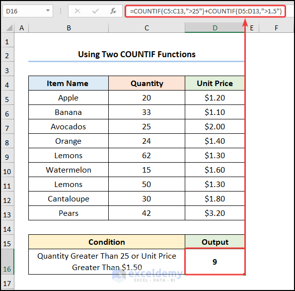
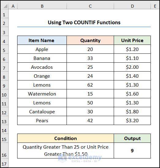
The results should look like the figure shown below.
Method 2 – Combining SUMPRODUCT and COUNTIF Functions
Steps:
- Move to the D16 cell >> type in the expression given below.
=SUMPRODUCT(COUNTIF(D5:D13,{"<1.50",">2.00"}))
The D5:D13 cells represent the Unit Price column.
Formula Breakdown:
- COUNTIF(D5:D13,{“<1.50″,”>2.00″}) → counts the number of cells within a range that meet the given condition. Here, the D5:D13 cells represent the range argument that refers to the Unit Price, while the {“<1.50″,”>2.00″} indicates the criteria argument that returns the count of the values in between the range $1.5 to $2.00.
- Output → {5,1}
- SUMPRODUCT(COUNTIF(D5:D13,{“<1.50″,”>2.00″})) → becomes
- SUMPRODUCT({5,1}) → returns the sum of the products of corresponding ranges or arrays. {5,1} is the array1 argument which refers to the number of instances returned by the COUNTIF function.
- Output → 6
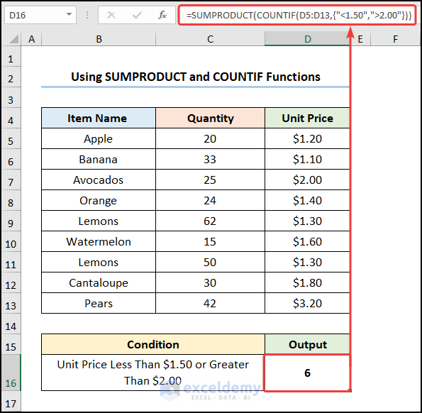
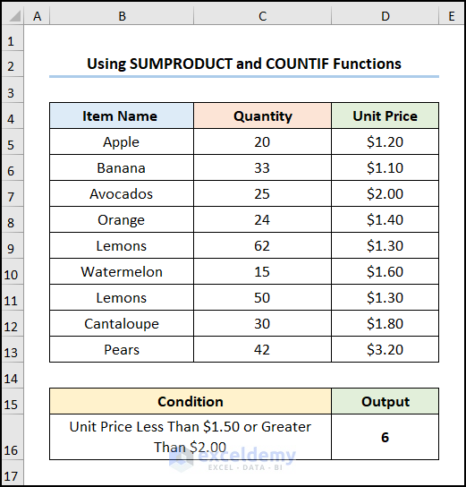
The results should look like the image shown below.
Method 3 – Using IF and COUNTIF Functions
Steps:
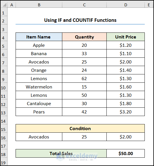
- Navigate to the D18 cell >> copy and paste the equation given below.
=IF(COUNTIF($B$5:$B$13,B16),C16*D16,"Not Available")
The B16, C16, and D16 cells point to Avocados, 25, and $2.00 respectively.
Formula Breakdown:
- COUNTIF($B$5:$B$13,B16) → The $B$5:$B$13 cells represent the range argument that refers to the Item Name, while the B16 cell indicates the criteria argument that is Avocados.
- Output → 1
- IF(COUNTIF($B$5:$B$13,B16),C16*D16,”Not Available”) → becomes
- IF(1,C16*D16,”Not Available”) → checks whether a condition is met and returns one value if TRUE and another if FALSE. Here, 1 is the logical_test argument, which prompts the IF function to return C16*D16 (value_if_true argument) it returns “Not Available” (value_if_false argument).
- Output → $50.00
Note: Please make sure to use Absolute Cell Reference by pressing the F4 key on your keyboard.
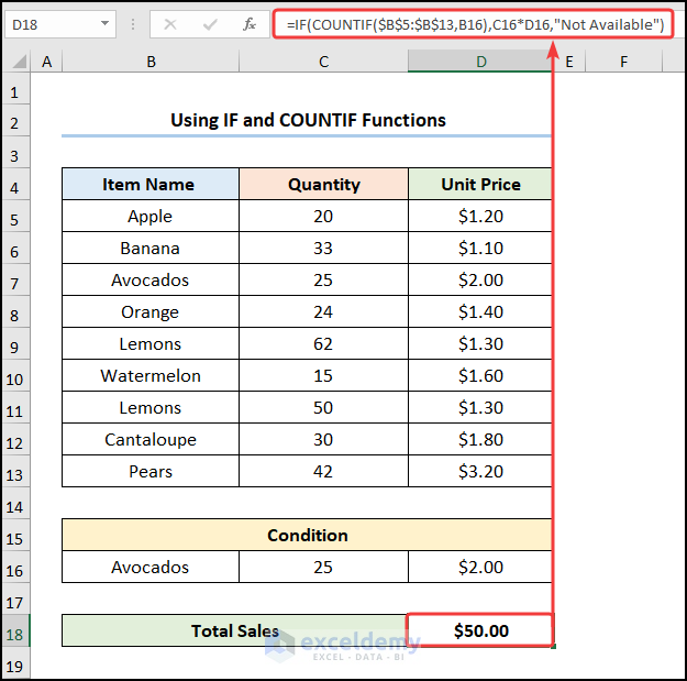
Your output should look like the picture given below.
Method 4 – Utilizing SUM and COUNTIFS Functions
Steps:
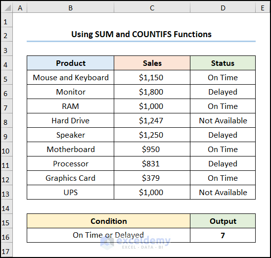
- Jump to the D16 cell >> insert the expression into the Formula Bar.
=SUM(COUNTIFS($D$5:$D$13, {"On Time","Delayed"}))
The D5:D13 cells indicate the delivery Status column.
Formula Breakdown:
- COUNTIFS($D$5:$D$13, {“On Time”,”Delayed”}) → counts the number of cells specified by a given set of conditions and criteria. The $D$5:$D$13 cells represent the criteria_range1 argument that refers to the Status, whereas the “<>” indicates the criteria1 argument the criteria On Time and Delayed.
- Output → {4,3}
- SUM(COUNTIFS($D$5:$D$13, {“On Time”,”Delayed”})) → becomes
- SUM({4,3}) → adds all the numbers in a range. Here, {4,3} is the number1 argument which refers to the output returned by the COUNTIFS function.
- Output → 7
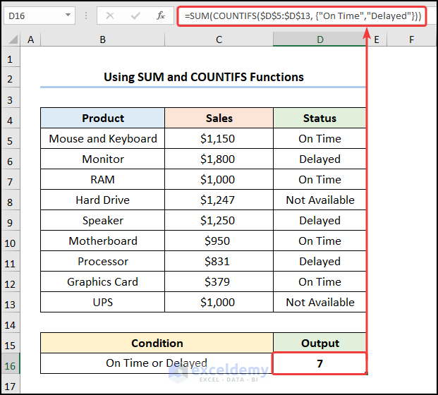
The final output should look like the screenshot shown below.
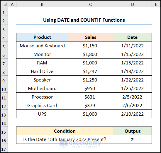
Method 5 – Employing DATE and COUNTIF Functions
Steps:
- Enter the following into the D16 cell.
=COUNTIF($D$5:$D$13,DATE(2022,1,15))
The D5:D13 range of cells represents the Date column.
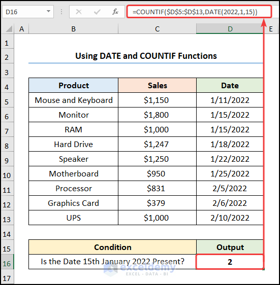
This yields the output shown in the figure below.
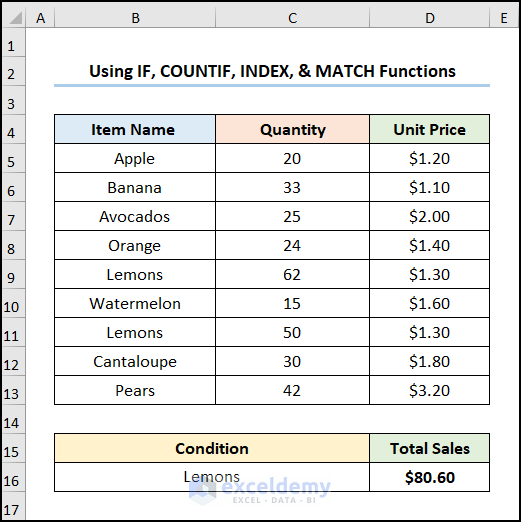
Method 6 – Applying COUNTIF, IF, INDEX, and MATCH Functions
Steps:
- Enter the D16 cell >> type in the following expression
=IF(COUNTIF($B$5:$B$13, B16),INDEX($C$5:$C$13, MATCH(B16, $B$5:$B$13,0))*INDEX($D$5:$D$13, MATCH(B16, $B$5:$B$13,0)), "")
The B16 cell points to the condition Lemons.
Formula Breakdown:
- MATCH(B16, $B$5:$B$13,0) → returns the relative position of an item in an array matching the given value. B16 is the lookup_value argument that refers to the Condition Lemons. Following, $B$5:$B$13 represents the lookup_array argument from where the value is matched. 0 is the optional match_type argument which indicates the Exact match criteria.
- Output → 5
- INDEX($C$5:$C$13, MATCH(B16, $B$5:$B$13,0)) → becomes
- =INDEX($C$5:$C$13,5) → returns a value at the intersection of a row and column in a given range. The $C$5:$C$13 is the array argument which is the Quantity. Lastly, 5 is the row_num argument that indicates the row location.
- Output → 62
- IF(COUNTIF($B$5:$B$13, B16),INDEX($C$5:$C$13, MATCH(B16, $B$5:$B$13,0))*INDEX($D$5:$D$13, MATCH(B16, $B$5:$B$13,0)), “”) → becomes
- IF(2,62*1.3,””) → 2 is the logical_test argument which prompts the IF function to return 62*1.3 (value_if_true argument) otherwise it returns “” (Blank) (value_if_false argument).
- Output → $80.60
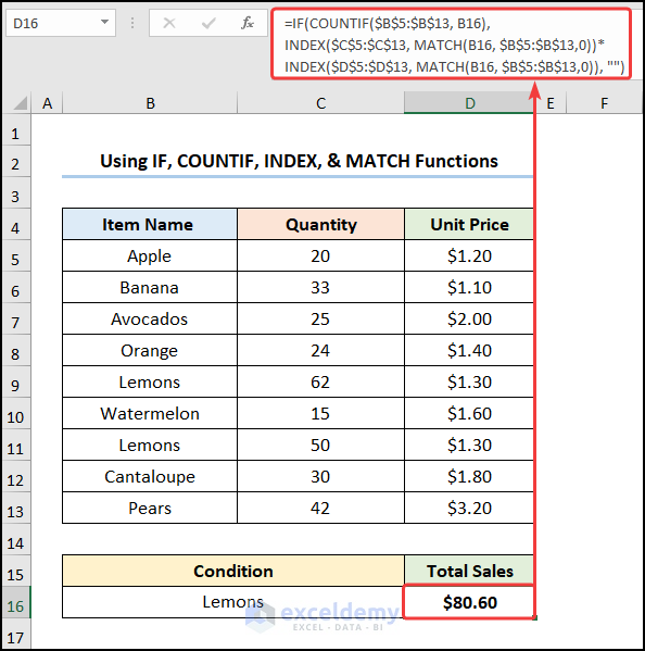
The results should appear in the image below.
How to Use COUNTIF with Multiple Criteria in the Same Column in Excel
Steps:
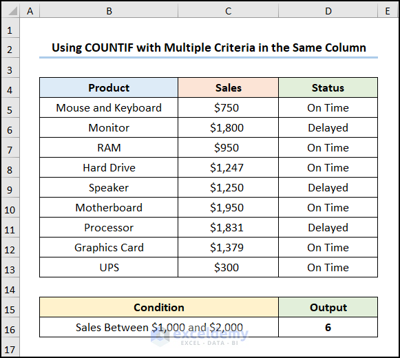
- Insert the equation in the D16 cell as shown below.
=COUNTIF($C$5:$C$13, ">1000")-COUNTIF($C$5:$C$13,">2000")
The C5:C13 array represents the Sales column.
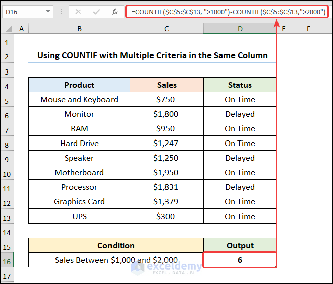
The output should be 6, as shown in the screenshot below.
We skipped some of the relevant Examples of the COUNTIF function with multiple criteria in the same column, which you might explore if you want.
How to Use COUNTIFS with Multiple Criteria in Different Columns in Excel
Steps:
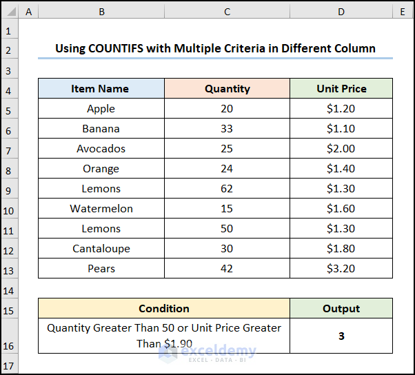
- Navigate to the D16 cell and insert the expression below.
=COUNTIFS($C$5:$C$13,">50")+COUNTIFS($D$5:$D$13,">1.9")
The C5:C13 and D5:D13 arrays refer to the Quantity and Unit Price.
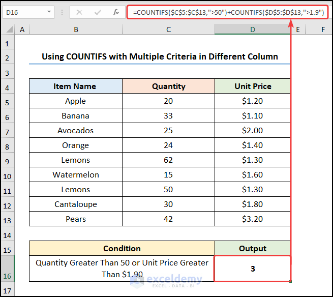
The final output should appear in the picture below.
We skipped some relevant Examples of the COUNTIFS with multiple criteria in different columns, which you may explore if you wish.
Download Practice Workbook
<< Go Back to Excel COUNTIF Function | Excel Functions | Learn Excel
Get FREE Advanced Excel Exercises with Solutions!
