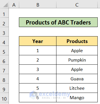
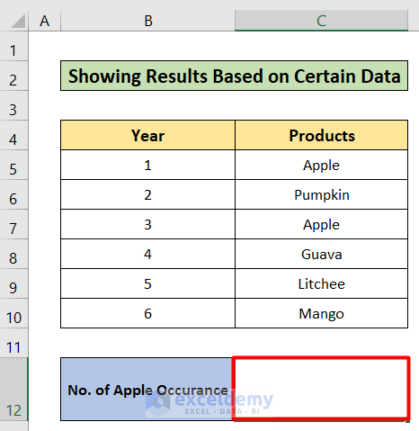
Let’s consider the following dataset about the Products of ABC Traders. The dataset has two columns, B and C, called Year and Products. The dataset ranges from B4 to C10. I will use this dataset to show the IF and COUNTIF functions together in Excel with 5 suitable methods.
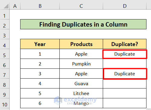
Method 1 – Using a Combination of IF and COUNTIF Functions to Find Duplicates in a Column
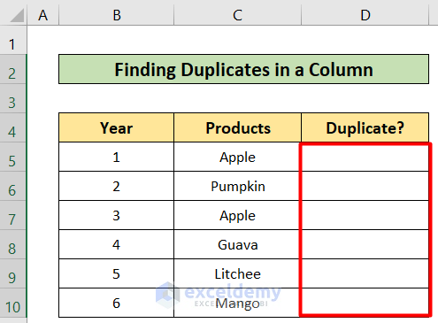
Steps:
- Select cell D5.
- Copy the following formula to the selected cell:
=IF(COUNTIF($C$5:$C$10,C5)>1,"Duplicate","")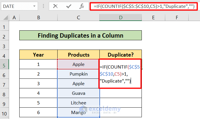
- Press Enter to get the following results:
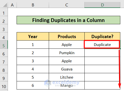
- Copy the formula from D5 to D10.
How Does the Formula Work?
- COUNTIF($C$5:$C$10,C5): This part of the formula counts the value of C5 in the range of C5 to C10.
- IF(COUNTIF($C$5:$C$10, C5)>1, “Duplicate”,””): Now, the returned value from the COUNTIF formula checks the argument. If the returned value is greater than 1, the IF function will return the “Duplicate” text. Otherwise, nothing will be returned.
Read More: How to Use COUNTIF and COUNTA Functions Together in Excel
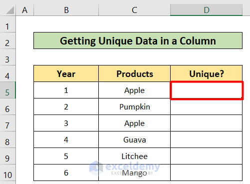
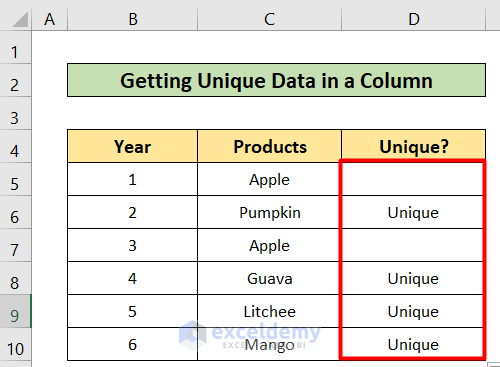
Method 2 – Applying IF and COUNTIF Functions to Get Unique Data in a Column
Steps:
- Select cell D5.
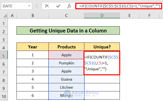
- Copy the following formula in the D5 cell:
=IF(COUNTIF($C$5:$C$10,C5)=1,"Unique","")
- Press Enter to get the following result:
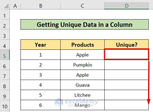
- Fill handle the formula from the C5 to C10 cells.
How Does the Formula Work?
- COUNTIF($C$5:$C$10,C6): This part of the formula counts the value of C5 in the range of C5 to C10.
- IF(COUNTIF($C$5:$C$10, C5)=1, “Unique”,””): Now, the returned value from the COUNTIF formula checks the argument. If the returned value is equal to 1, the IF function will return “Unique” text. Otherwise, nothing will be returned.
Read More: How to Use the Combination of COUNTIF and SUMIF in Excel
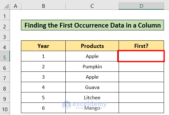
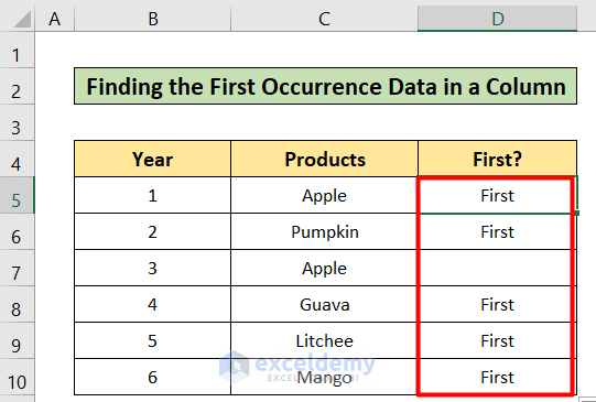
Method 3 – Inserting IF and COUNTIF Functions Together to Find the First Occurrences of Data in a Column
Steps:
- Select cell D5.
- Copy the following formula in the selected cell and press Enter:
=IF(COUNTIF($C$5:C5,C5)=1,"First","")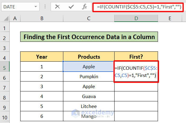
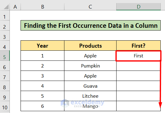
- Copy the formula from the D5 to D10 cells.
How Does the Formula Work?
- COUNTIF($C$5:C5, C5)=1: This part of the formula counts the value of C5 in the range of C5 to C10.
- IF(COUNTIF($C$5:C5, C5)=1, “First”,””): Now, the returned value from the COUNTIF formula checks the argument. If the returned value is equal to 1, the IF function will return the “First” text. Otherwise, nothing will be returned.
Read More: How to Use Nested COUNTIF Function in Excel
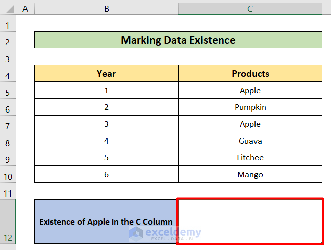
Method 4 – Combining IF and COUNTIF Functions to Mark Data Existence
Steps:
- Select cell C12.
- Copy the following formula in the selected cell:
=IF(COUNTIF(C5:C10, "Apple")>0, "Exists", "Doesn't Exist")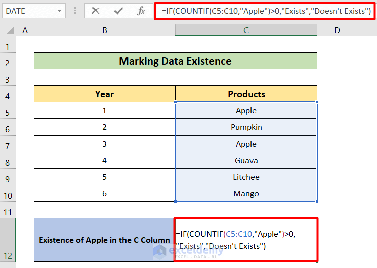
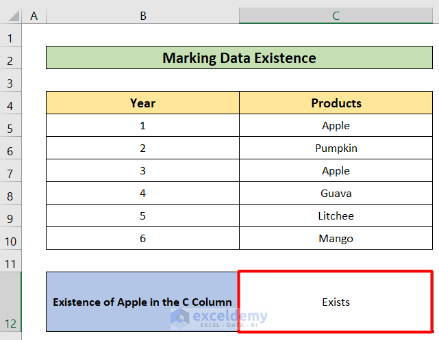
- Press the Enter button.
How Does the Formula Work?
- COUNTIF(C5:C10, “Apple”): This part of the formula counts the value “Apple” in the range of C5 to C10.
- IF(COUNTIF(C5:C10, “Apple”)>0, “Exists”, “Doesn’t Exist “): Now, the returned value from the COUNTIF formula checks the argument. If the returned value is greater than 0, the IF function will return the “Exists” text. Otherwise, “Doesn’t Exist” will be returned.
Read More: Difference Between SUMIF and COUNTIF Functions in Excel
Method 5 – Applying IF and COUNTIF Functions Together to Show Results Based on the Amount of Certain Data
Steps:
- Select cell C12.
- Copy the following formula in the C12 cell:
=IF(COUNTIF(C5:C10, "Apple")=0, "0", IF(COUNTIF(C5:C10, "Apple")=1, "One", "Multiple"))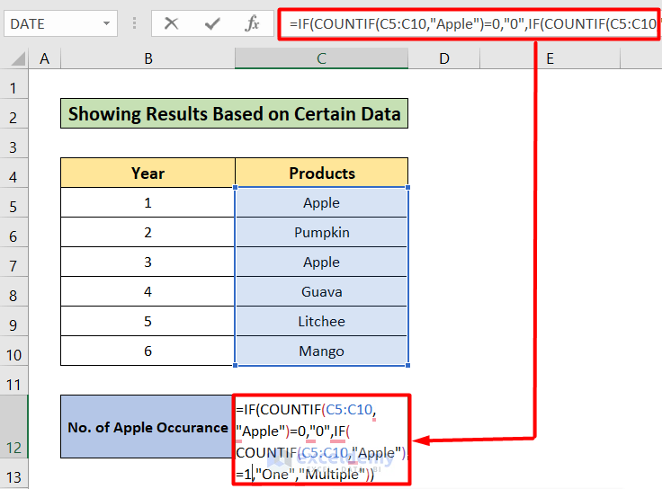
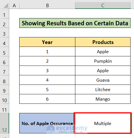
- Press Enter to get the result pictured below:
How Does the Formula Work?
- COUNTIF(C5:C10, “Apple”): This part of the formula counts the value “Apple” in the range of C5 to C10.
- IF(COUNTIF(C5:C10, “Apple”)=0, “0”, IF(COUNTIF(C5:C10, “Apple”)=1, “One”, “Multiple”)): Now, the returned value from the COUNTIF formula checks the argument. If the returned value is equal to 0, the IF function will return the “0” text. As for the next COUNTIF function, if the returned value is equal to 1, the IF function will return the “One” text. Otherwise, “Multiple” will be returned.
Read More: How to Use SUMIF, COUNTIF and AVERAGEIF Functions in Excel
Things to Remember
- As the fifth formula is a big one, you need to be careful when giving input on the values and arguments.
Download Practice Workbook
Feel free to download the following workbook to practice on your own.
<< Go Back to Excel COUNTIF Function | Excel Functions | Learn Excel
Get FREE Advanced Excel Exercises with Solutions!

is something like this possible?
IF(COUNTIFS(R2,”value1*”,S2,”status1″),”aaa”,”bbb”),IF(COUNTIF(R6,”value2*”),”aaa”,”bbb”)
or
IF(COUNTIFS(R2,”value1*” OR “value2″,S2,”status1” OR “status2” or “status3″),”aaa”,”bbb”)
Thanks
Dear EMMA PALMER,
Greetings. Thank you for your question. I have provided a primary solution to your question. It would be much easier for me to solve your problem if you could send me your dataset and Excel workbook.
Yes, it is feasible to use both of the formulas you gave. However, your usage of syntax is not totally accurate. The proper syntax for each formula is as follows:
Formula 1:
=IF(COUNTIFS(R2,”value1*”,S2,”status1″),”aaa”,”bbb”)
This formula checks if the value in cell R2 starts with “value1” and the value in cell S2 is “status1”. If both conditions are true, it returns “aaa”; otherwise, it returns “bbb”.
Formula 2:
=IF(OR(COUNTIF(R2,”value1*”), COUNTIF(R2,”value2*”)), “aaa”, “bbb”)
This formula checks if the value in cell R2 starts with either “value1” or “value2”. If either condition is true, it returns “aaa”; otherwise, it returns “bbb”.