Method 1 – Application of SUMIF Function in Excel
⏩ Overview of SUMIF Function
The SUMIF function is used for summing numerical values based on criteria assigned over a specific range. The syntax of this function is:
=SUMIF (range, criteria, [sum_range])
Here, in the function, range means the cells in which criteria are to be assigned, and the sum_range is the range in which value is to be calculated. Criteria may be numbers, cell references, text, or output of other functions.
Application
For the dataset we are dealing with, multiple companies are selling Glass at different prices. We want to find out the Total Price of the Glass using the SUMIF function. As this function sums value on a given criterion, we also want to calculate the total prices of all items greater than $2000.
Steps:
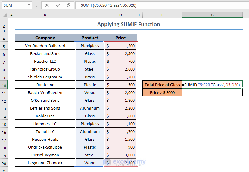
- Select a cell where you want to find out the Total Price of Glass. Type the formula stated below in that cell.
=SUMIF(C5:C20,"Glass",D5:D20)
Here,
- C5:C20 = The range on which criteria to be assigned
- Glass = Criteria (As we only want the total price of Glass)
- D5:D20 = sum will be calculated from this range
Formula Unlocking
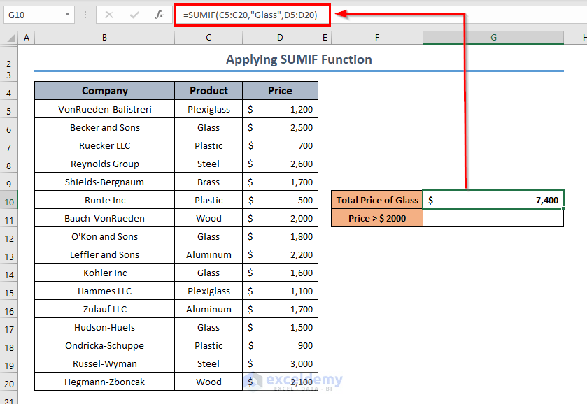
The function looks for the criteria: Glass in the range C5:C20. Then it finds the cells where the criteria are met and sums the cell from the range D5:D20.
- Press ENTER, and this cell will calculate the Total price of Glass.
This formula has used descriptive or text criteria.
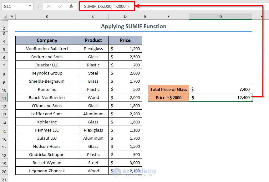
If you want to assign a numerical criterion to your dataset, Excel also keeps the door open. We want to calculate the Total of the prices which are Greater than $2000. Apply the following formula to get the sum of prices exceeding $2000.
=SUMIF(D5:D20,">2000")
Method 2 – Using the COUNTIF Function in Excel
⏩ Overview of COUNTIF Function
The objective of the COUNTIF function is to count the number of cells with a range based on a given criterion.
The syntax of this function is:
=COUNTIF(range, criteria)
The range is a compulsory argument where criteria are assigned and from which cells will be counted. The criteria may be text or numerical.
Application
The same set of data will be used now for demonstrating the application of the COUNTIF function. In the datasheet, you may notice that products are found repeat for different companies. If you want to find the number of companies that sell a specific product (i.e. Glass), you should count how many times that product occurred in the data set.
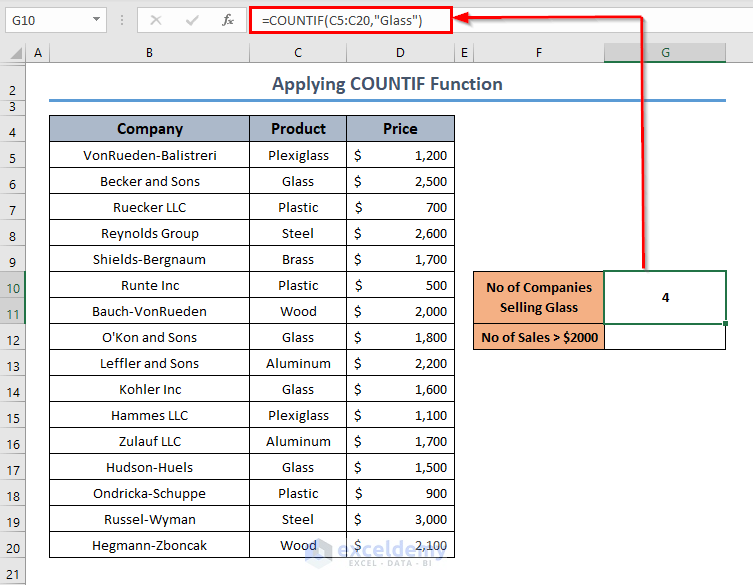
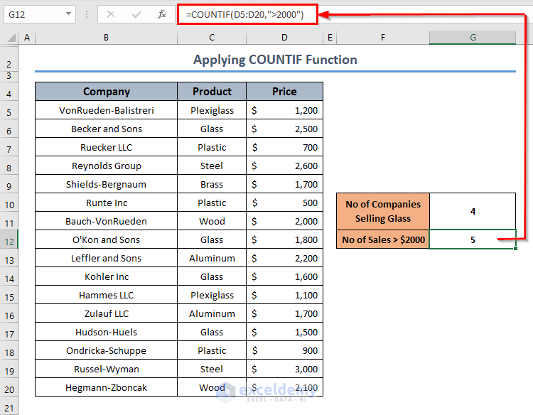
To count the total number of companies selling a similar product (i.e. Glass), apply the formula below.
=COUNTIF(C5:C20,"Glass")
- C5:C20 = The range on which criteria to be assigned
- Glass = Criteria (As we only want the total price of Glass)
The function counts the cells where this criterion is met and returns it to the formulated cell.
You can also count specific data on a Numerical Criterion, like the number of sales greater than $2000. Just apply the formula in the form stated below.
=COUNTIF(D5:D20,">2000")
The criteria is set “>2000”.So, the function counts all the cells in the range D5:D20 and returns the counted result.
Method 3 – Appliance of AVERAGEIF Function in Excel
⏩ Overview of AVERAGEIF Function
The AVERAGEIF function is a special Excel function used for calculating the arithmetic mean or the average of some numerical values based on a specified condition or criterion. The syntax of this function is:
=AVERAGEIF(range, criteria, [average_range])
The first argument range describes the cells where the condition is to be applied and the criteria denote the condition for the range. The range from which the average value is to be calculated is the average_range.
Application
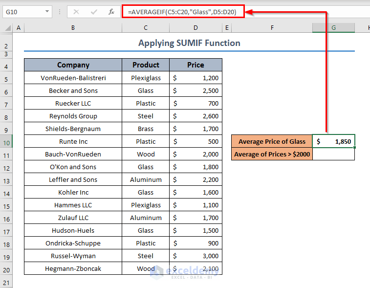
Previously, we counted the number of companies (4) selling a similar product: glass, and the total price for this product was also calculated (i.e. $7400). Dividing the total price by number will get you the average value. But if you want to calculate the average value directly from the dataset, apply the following formula.
=AVERAGEIF(C5:C20,"Glass",D5:D20)
The function meets the criterion Glass in the range C5:C20 and extracts value from the range D5:D20. It calculates the averages of the extracted value.
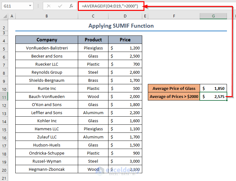
The AVERAGEIF function takes the criteria into consideration. The criteria may be of numerical condition also. If you want to calculate the average of some numbers greater than (i.e. >$2000), use the following formula.
=AVERAGEIF(D4:D19,">2000")
It finds all the cells from the range D4:D19 and calculates the average of those values.
Download Practice Workbook
You can download the practice book from the link below.
Related Articles
- How to Use Nested COUNTIF Function in Excel
- How to Use COUNTIF and COUNTA Functions Together in Excel
<< Go Back to Excel COUNTIF Function | Excel Functions | Learn Excel
Get FREE Advanced Excel Exercises with Solutions!
