The SUMIF Function in Excel – Quick View
Introduction to the Excel SUMIF Function:
Summary:
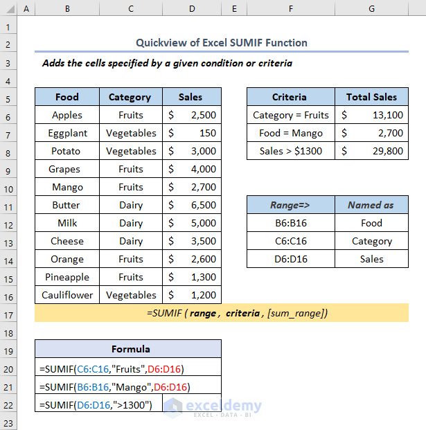
This function adds the cells specified by a given condition or criteria.
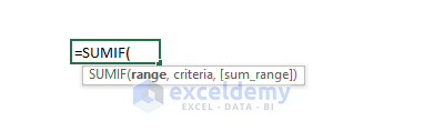
Syntax:
Arguments:
| Argument | Required/Optional | Explanation |
|---|---|---|
| range | Required | The range of cells to evaluate by criteria. |
| criteria | Required | The criteria: an expression, a number, a text, a function, or a cell reference that defines which cells to add. |
| sum range | Optional | The cells to add to combine cells that are not defined in the range argument. |
Note:
- In the criteria, wildcard characters can be included: a question mark (?) to match a single character, an asterisk (*) to match a sequence of characters. Like 6?”, “apple*”, “*~?”
- sum_range should be the same size and shape as the range.
- The SUMIF function can only have a single condition.
Example 1 – Calculating a Sum with Numeric Criteria Using the SUMIF Function
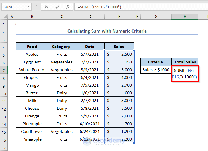
To count the total sales whose price was more than $1000 in H7.

- Enter the formula in H7.
=SUMIF(E5:E16,">1000")E5:E16 refers to the Sales column.
Formula Breakdown:
- E5:E16 is the range for the sum operation.
- “>1000” is the criteria. If the sales value is more than $1000, it will be counted. Otherwise, it will be ignored.
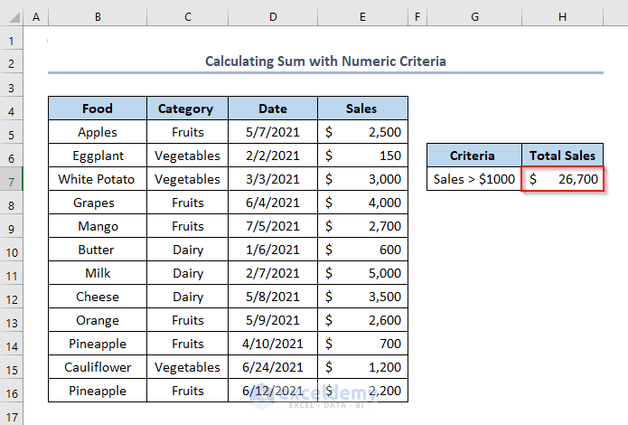
- Press ENTER.
The output is $26,700.
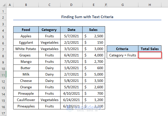
Example 2 – Finding a Sum with Text Criteria Using the SUMIF Function
Calculate the sales in the Fruits Category.
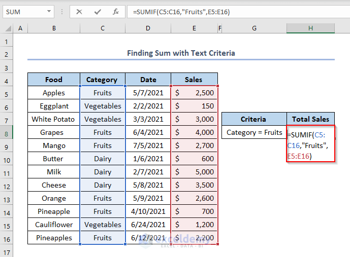
- Enter the formula in H8.
=SUMIF(C5:C16,"Fruits",E5:E16)Formula Breakdown:
- C5:C16 is the range to check the criteria.
- “Fruits” is the condition or criteria. It checks if the Category is Fruits.
- E5:E16 is the sum range.
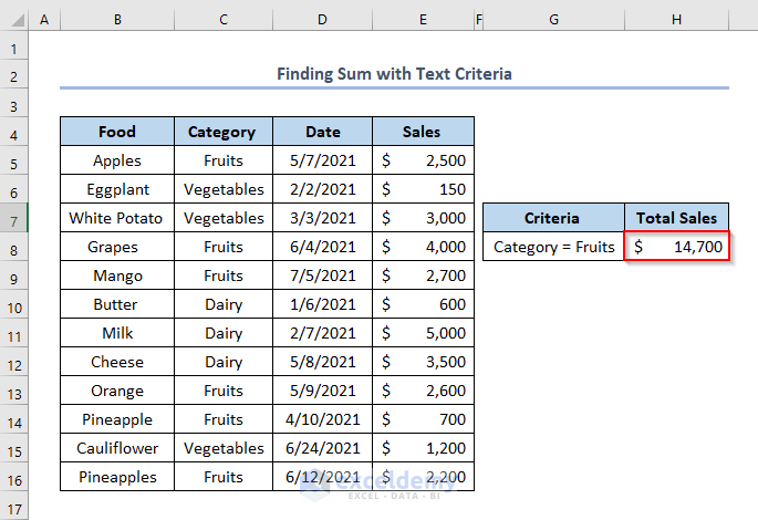
- Press ENTER.
The output is $14,700.
Read More: Excel SUMIFS with Not Equal to Text Criteria
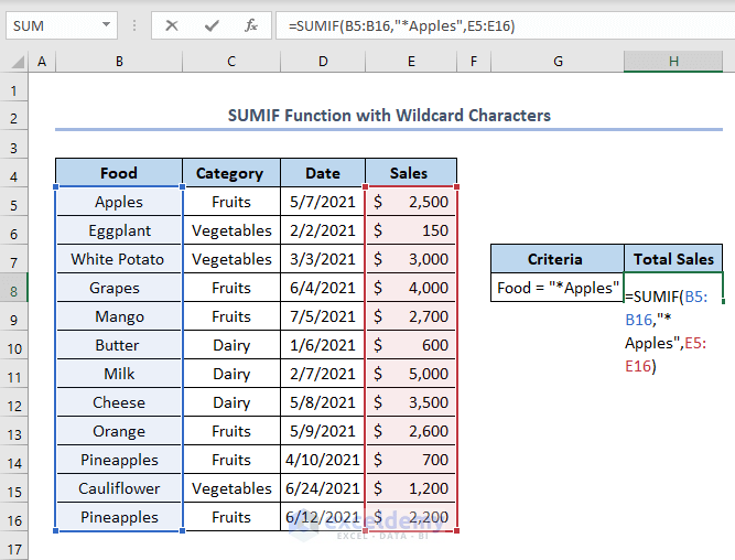
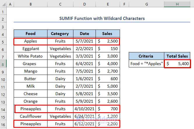
Example 3 – Use the SUMIF Function with Wildcard Characters for a Partial Match
To calculate the total sales of Apples.
- Enter the formula in H8.
=SUMIF(B5:B16,"*Apples",E5:E16)Formula Breakdown:
- “*Apples” will find the name Apples or a name in which the first or last part is apples.
- Press ENTER to see the output.
Read More: [Fixed!] Excel SUMIF with Wildcard Not Working
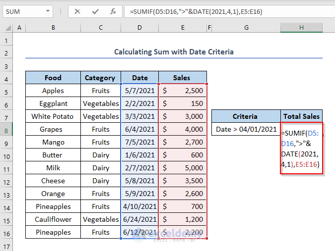
Example 4 – Calculating the Sum with Date Criteria
To get the sales of foods sold after 04/01/2021.
- Enter the formula in H8.
=SUMIF(D5:D16,">"&DATE(2021,4,1),E5:E16)Formula Breakdown:
- “>”&DATE(2021,4,1) is the criteria. “>” is used to find the greater dates. The ampersand (&) is used to concatenate the formula and text. The DATE function is used to give the date input.
- The DATE function accepts three arguments: year, month, and day. (If you want to know more about this function you can check this Link)
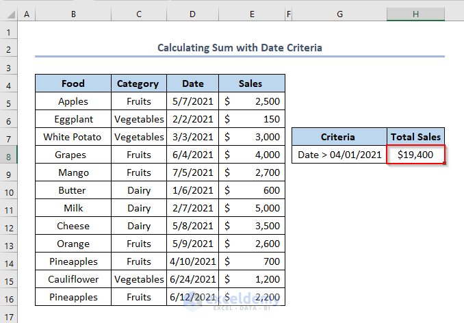
- Press ENTER.
This is the output.
Read More: Excel SUMIF with Date Range
Example 5 – Calculating the Sum with the OR Criteria in the SUMIF Formula
To calculate the total sales of Vegetables, or sales greater than $1000.
- Enter the formula in H8.
=SUMIF(C5:C13,"Vegetables",E5:E16)+SUMIF(E5:E13,">1000",E5:E16)-SUMIFS(E5:E16,C5:C16,"Vegetables",E5:E16,">1000")
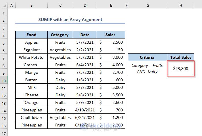
Example 6 – Applying the SUMIF with a Criteria Array
To count the total sales in the Category Fruits and Dairy:
- Enter the formula in H8.
=SUM(SUMIF(C5:C16,{"Fruits","Dairy"},E5:E16))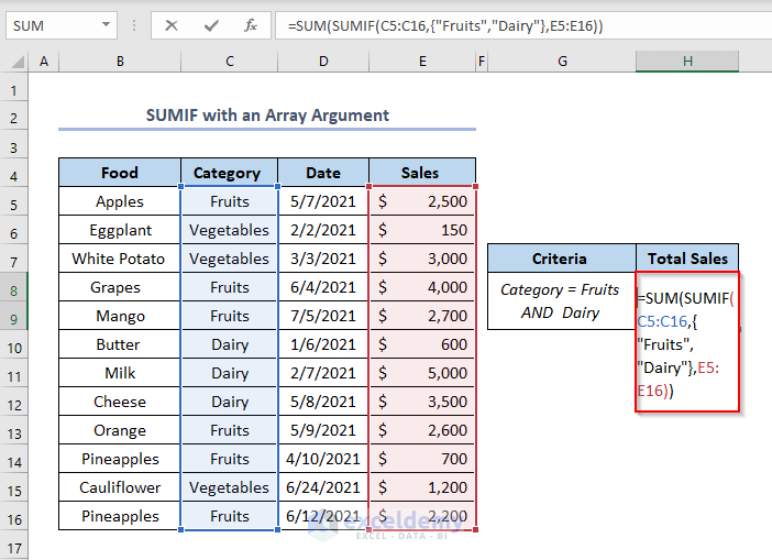
- Press ENTER.
This is the output.
Read More: How to Use 3D SUMIF for Multiple Worksheets in Excel
Example 7 – Using the SUMIF with Date Range (Month and Year) Criteria
Find the Total Bill.
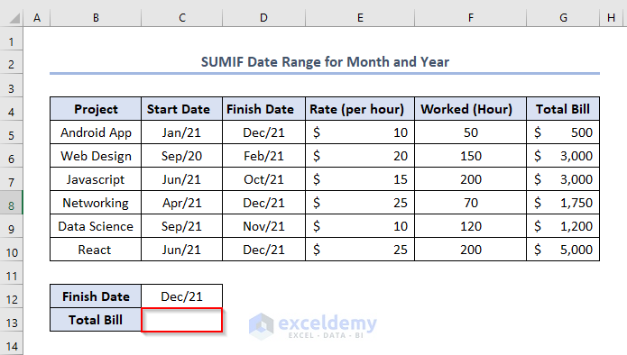
- Enter the formula in C13.
=SUMIF(D5:D10,"="&C12,G5:G10)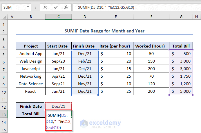
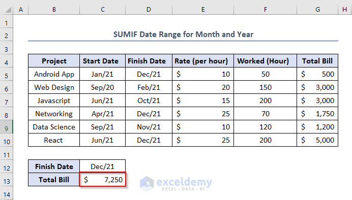
- Press ENTER.
This is the output.
Read More: [Fixed] Excel SUMIF Not Working
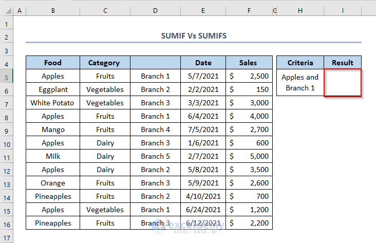
SUMIF Vs SUMIFS in Excel: What’s the Difference?
Both the SUMIF and SUMIFS function add the values of all cells in a range that meet a given criterion, but:
- The SUMIF function adds all cells in the range that match particular criteria.
- The SUMIFS function counts how many cells in a range meet a set of criteria.
To find Sales of Apples in Branch 1:
- Enter the formula in I5.
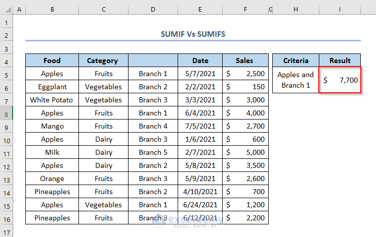
=SUMIFS(F5:F16,B5:B16,"Apples",D5:D16,"Branch 1")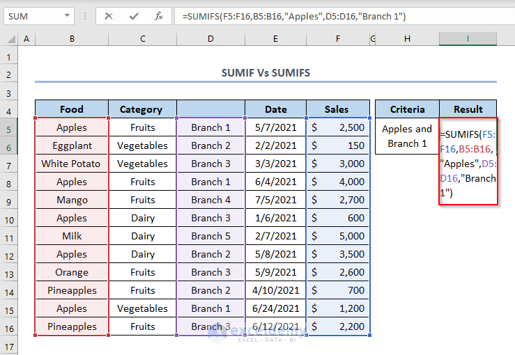
- Press ENTER.
This is the output.
The SUMIF function finds the finish date Dec-21, and calculates the total bill.
Things to Remember
The SUMIF function returns incorrect results (#VALUE! error) when you use it to match strings longer than 255 characters.
Download Practice Workbook
Excel SUMIF Function: Knowledge Hub
<< Go Back to Excel Functions | Learn Excel
Get FREE Advanced Excel Exercises with Solutions!

Example 5 is wrong. You double-counted the vegetables that are > $1000. How do you _really_ do this?
Hello Peter S.,
Thank you for catching that. You were right—the original example could lead to double-counting. We’ve reviewed and corrected the example in the article to address the issue. We appreciate your feedback, as it helps us improve the accuracy of our content.
Regards,
ExcelDemy