Dataset Overview
Let’s take a dataset where a charitable organization named Save the Poor has a list of donations.
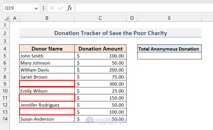
Here, in the Donor Name column, the blank cells represent those donors who want to stay anonymous. Now, we are interested in calculating the total anonymous donations, meaning we need to sum up the Donation Amounts next to the blank cells.
Method 1 – Summing Up the Total Run of Unnamed Donors
We can use the following formula, consisting of the SUMIF function, to sum up the anonymous donation amounts.
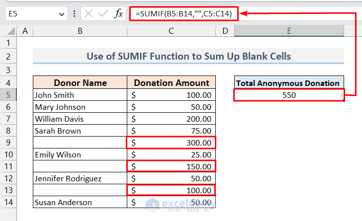
=SUMIF(B5:B14,"",C5:C14)
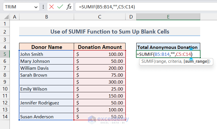
Click Enter to get the result.
How Does the Formula Work?
SUMIF(B5:B14,””,C5:C14)
Here,
- B5:B14: This is the range (Donor Name column) against which the criteria will be checked.
- “”: As we need to look for blank cells in the B5:B14 range, we set the argument empty inside inverted commas.
- C5:C14: Is the sum range (Donation Amount). The SUMIF function only sums those cells in the range C5:C14, where the corresponding cells in B5:B14 are blank.
Method 2 – Summing Up Pseudo Blank Cells Using the Trim Function and Helper Column
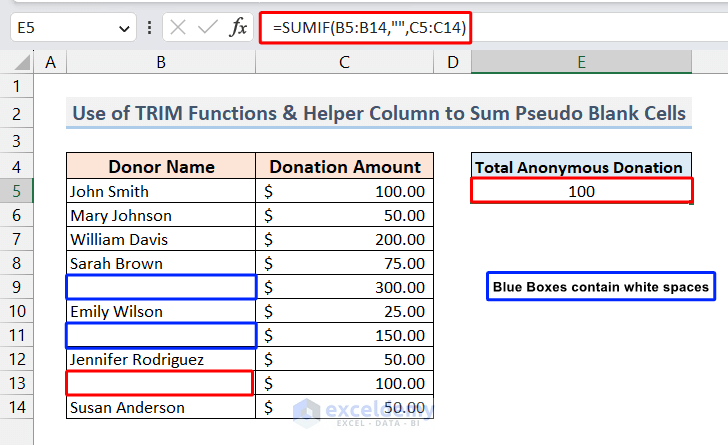
Sometimes we need to sum up values corresponding to cells that look blank or empty, but in reality, they contain white spaces. It can happen due to improper data extraction from other sources into Excel. For illustration, here we introduce some white spaces in the first two of three blank cells that we saw in the previous example. The SUMIF function will only take the last truly blank cell and display 100 as a result.
- To correct the result, we need to trim the whitespace using the TRIM function and store the result in a separate Helper Column.
=TRIM(B5)
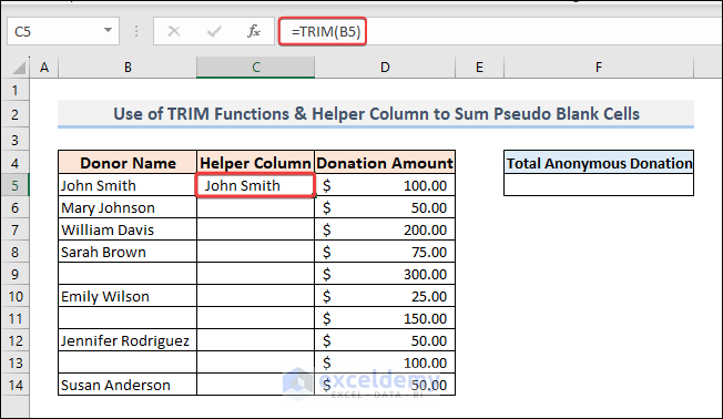
In the above picture, we can see that we have used the TRIM function in cell C5 to remove the white spaces from both ends of the text (leading and trailing spaces).
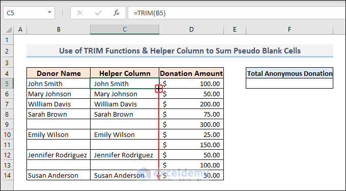
- Use the Fill Handle feature to autofill the rest of the cells from C6 to C14.
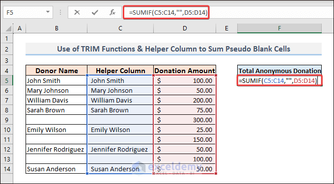
- Apply the SUMIF function while using the Helper Column as the criteria range in cell F5:
=SUMIF(C5:C14,“”,D5:D14)
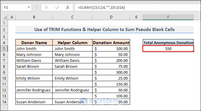
We will get our desired result, which is 550.
Alternative: Summing Up Pseudo Blank Cells Without the Helper Column
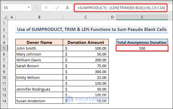
- Use the following formula consisting of the SUMPRODUCT, LEN, and TRIM functions to sum up the cells corresponding to all pseudo blank cells:
=SUMPRODUCT(--(LEN(TRIM(B5:B14))=0),C5:C14)

You will get the same result.
How Does the Formula Work?
- TRIM(B5:B14)
This function will trim off all the leading and trailing spaces (white spaces) from the range of cells B5:B14.
- LEN(TRIM(B5:B14))=0
This will logically test whether any cell from the range B5:B14 has a length of 0 (blank). It will return True for blank cells and False for non-blank cells.
- (–(LEN(TRIM(B5:B14))=0)
The double dash (–) converts the Trues and Falses into 1s and 0s, respectively.
- SUMPRODUCT(–(LEN(TRIM(B5:B14))=0),C5:C14)
The SUMPRODUCT function will multiply each element of the 1st array consisting of 1s and 0s with the corresponding elements of the 2nd array, which consists of Donation Amount and then sum up all the products together.
Method 3 – Using VBA SUMIF to Sum Cells Corresponding to Blank Cells
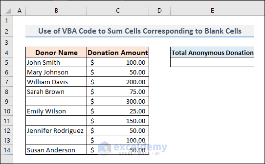
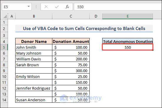
In this example, we will apply a VBA code in cell E5 to sum cells corresponding to blank cells.
Copy and paste the VBA code:
- Open the VBA Editor by clicking ALT+F11.
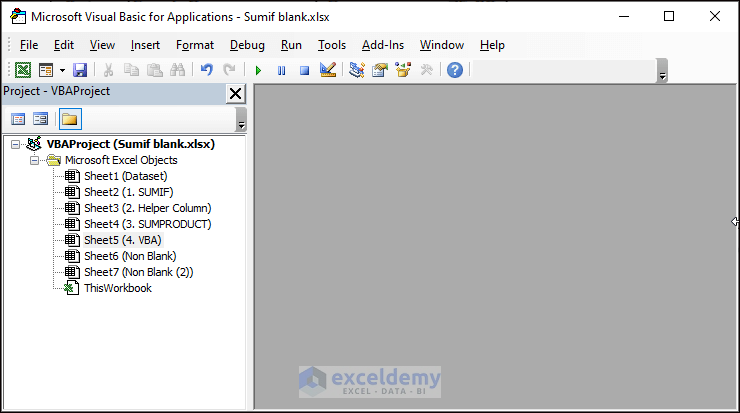
- Click the left button on the mouse on the sheet name to open the sheet module.
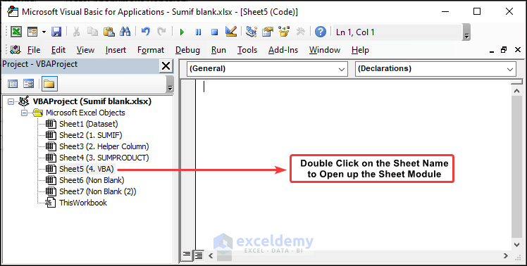
- Copy and paste the following code:
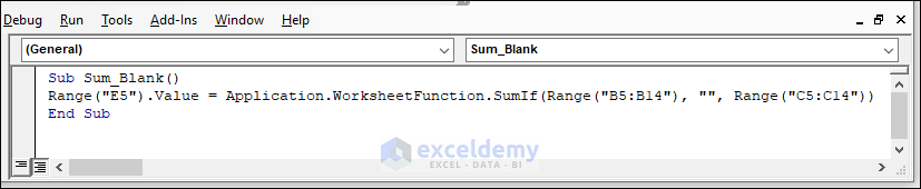
VBA Code Syntax:
Sub Sum_Blank()
Range("E5").Value = Application.WorksheetFunction.SumIf(Range("B5:B14"), "", Range("C5:C14"))
End Sub
- Run the code by clicking F5. You will see the desired result in cell E5.
How Does the Code Work?
The code utilizes the SumIf method of Application.WorksheetFunction.
The arguments of the SumIf method:
- The 1st argument Range(“B5:B14”) is the range where criteria will be checked.
- The 2nd argument “” implies that the method will look for blank/empty cells.
- The 3rd argument, Range(“C5:C14”) is the sum range.
The result is displayed in cell E5 of the worksheet.
Sum Values Based on Non-Blank Cells
If you want to sum cells corresponding to non-blank cells from the dataset that we have used in the 1st example, you can do that only by slightly modifying the formula as supplied below:
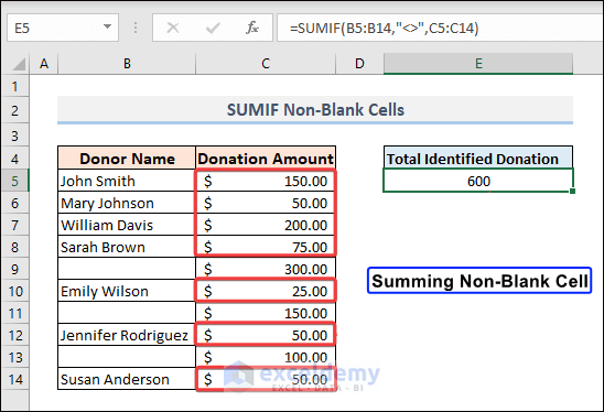
=SUMIF(B5:B14,"<>",C5:C14)
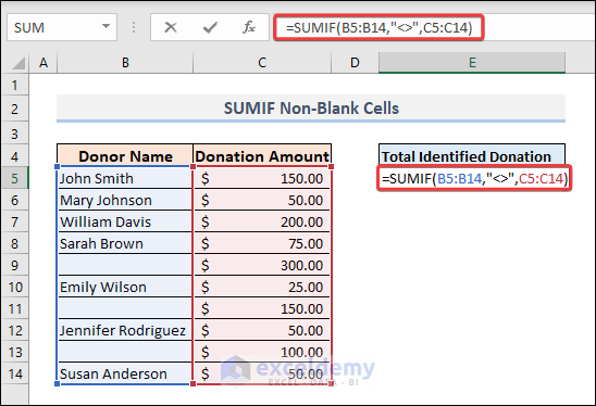
You will get the desired result.
How Does the Formula Work?
SUMIF(B5:B14,”<>”,C5:C14)
Here,
- B5:B14: the range is the criteria range against which the criteria will be checked.
- “<>”: Is the criterion that checks for non-blank cells.
- C5:C14: Is the sum range.
Read More: How to Use SUMIF Function to Sum Not Blank Cells in Excel
Excel Sums Blank Cells As Zero
On occasion, instead of displaying the result of a sum as 0, it may be more practical to display the result as a blank cell in Excel. In this section, we will learn how to display zero sum results as blank cells in Excel. For illustration, suppose we have four columns, and in the bottom cells, the sums are calculated.
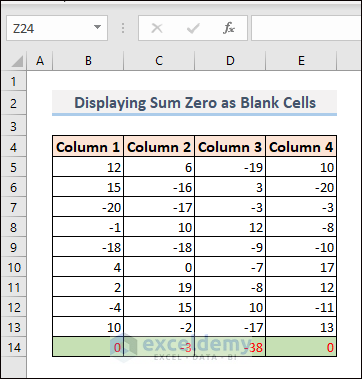
Here, we can see that B14 and E14 have 0 sum values. Now, our target is to display them as blank cells. To do that, follow the steps below.
Steps:
- Select the bottom row or the cells where you want to change the display format.
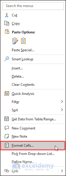
- Right-click on the mouse.
- The context menu will appear. From the context menu, click on Format Cells.
- A new window named Format Cells will appear.
- From the menu, click on Custom from the Category tab in the left corner.
- In the Type bar, write General;General;;@ .
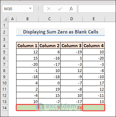
- Click OK.

- You will see that the cells that contained 0 are now displayed as blank cells.
Things to Remember
- Check for Pseudo Blank Cells:
- If your dataset contains white spaces or pseudo blank cells, follow the second method.
- Clean Dataset (No Pseudo Blank Cells):
- For a clean dataset without pseudo blank cells, use the first and third methods to accomplish your task.
Download Practice Workbook
You can download the practice workbook from here:
Related Articles
- Excel SUMIF Function for Not Equal Criteria
- Excel SUMIFS with Not Equal to Text Criteria
- Excel SUMIF Not Working
- [Fixed!] Excel SUMIF with Wildcard Not Working
<< Go Back to Excel SUMIF Function | Excel Functions | Learn Excel
Get FREE Advanced Excel Exercises with Solutions!
