Excel SUMIF Not Working (9 Possible Cases with Solutions)

With the help of Excel’s SUMIF function, users can sum a range of numbers in accordance with specific criteria. However, there are times when the SUMIF function may not work as expected, leading to incorrect results or no results at all. In this article, we will explore 9 reasons why the SUMIF function is not working in Excel and provide solutions to each of these reasons. We will discuss various potential issues and their fixes, ranging from incorrectly defined criteria arguments to problems with cell formatting. In addition, if the SUMIF function is not functioning at all, we will offer a different approach utilizing the SUMPRODUCT function. At last, you’ll get an output like the overview image below.

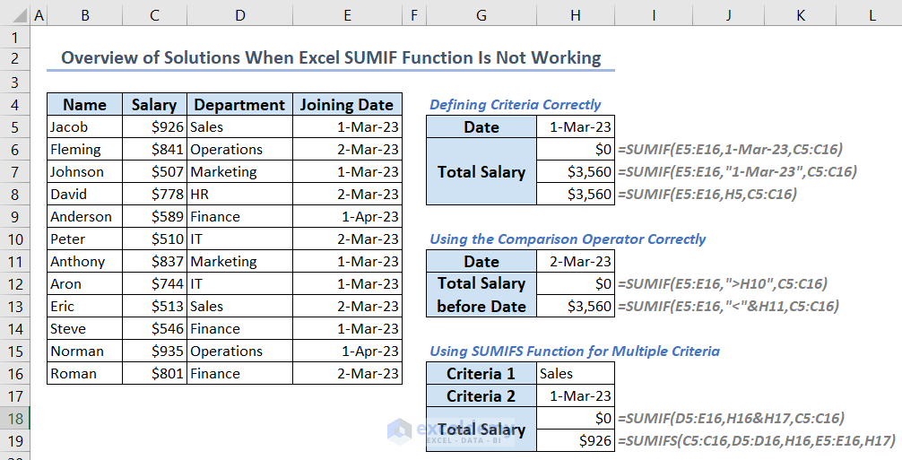
This image depicts 3 reasons and their solutions when the SUMIF function is not working among the 9 reasons we discussed in this article. Here you can see the solutions regarding defining criteria rightly, using the comparison operator correctly, and using the SUMIFS function for multiple criteria.

Introduction to SUMIF Function in Excel

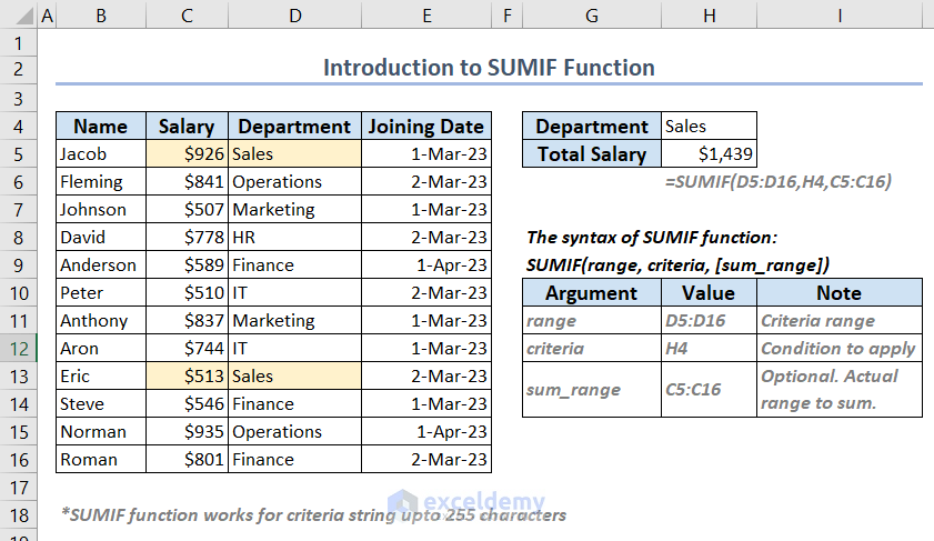
The SUMIF function adds numbers in a range that satisfies certain criteria. The syntax of the SUMIF function is:

In the following picture, you’ll get a full overview of the SUMIF function. Here we sum up the salaries of a few employees who are from the Sales department.

Excel SUMIF Function Not Working: 9 Reasons with Solutions

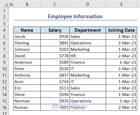
We are using the following dataset for showing you 9 reasons with solutions when the SUMIF function is not working in Excel. Here, we have some employee information from an organization. Their name, salary, respective department, and joining date can be found in this dataset.

1. Wrongly Defined Criteria Argument in SUMIF Function

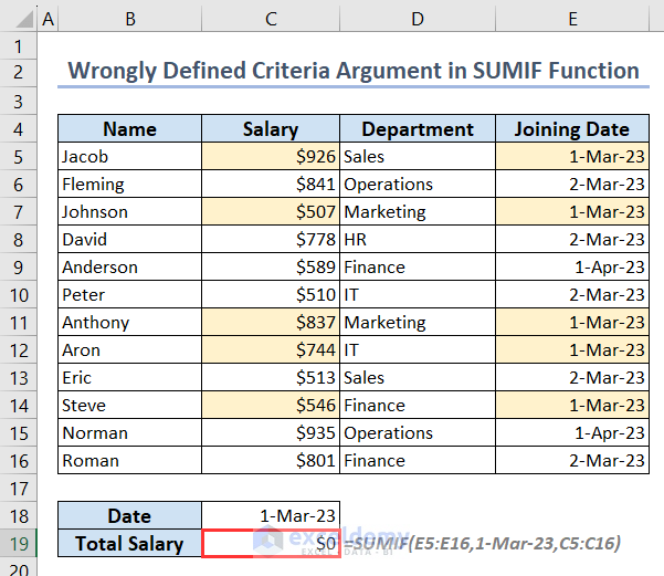
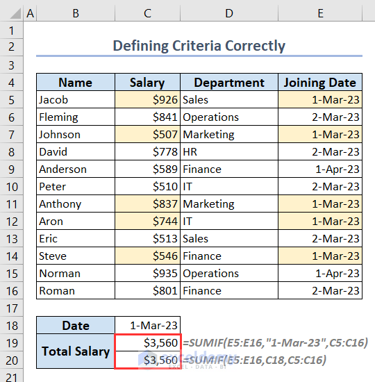
If you make a mistake during defining the criteria argument in the SUMIF function, you’ll not get any results. Depending on the situation, the SUMIF function’s criteria are specified differently. Like here we want to get the total salary of those employees who joined on the date 1-Mar-23.

• So, we put the following formula in cell C19:

• We have put the range as E5:E16 that are Joining Date column and sum range as C5:C16 that are Salary These 2 arguments are correct. But as we define the date criteria argument wrongly, it is giving 0 as a result.

Solution: Define Criteria Correctly

• To solve the issue, we have put the following 2 formulas, that will give the correct result.
• We put the first formula in cell C19:

• Now, we have put the date inside double quotations and the SUMIF function is working nicely. This happens because the SUMIF function takes the date as a text value, not a number value. So we have to insert it inside double quotations.
• We put another formula in cell C20:

• Here, we put the cell reference C18 directly as a criterion. So, we don’t have to worry about format.

2. Wrong Use of Comparison Operator in SUMIF Function

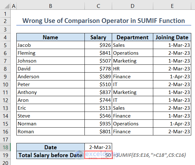
When you put the comparison operator wrongly into the Excel SUMIF function, you’ll see that the function is not working properly. Suppose, we want to get the total salary of those employees who joined before the date 2-Mar-23.

• We put the following formula in cell C19 and gets an incorrect result:

• Here we made 2 mistakes. We inserted the wrong comparison operator. It should be the less than operator (<). And the operator should reside inside double quotations alone and then the operator and the cell reference should join with an ampersand operator(&).

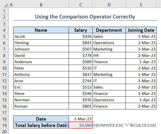
Solution: Use the Comparison Operator Correctly

• We put the correct formula in cell C19:

• Now, we put the correct operator, the less than operator (<) inside double quotations and join it with cell reference C18 with an ampersand operator(&).

Read More: [Fixed!] Excel SUMIF with Wildcard Not Working

3. Sum Range Is in Text Format

If the sum range is in text format, the SUMIF function can’t sum them. Because you can sum a range of numbers, not a range of text values. That’s why the following formula is giving 0 in cell C19 because the sum range C5:C16 is in text format:

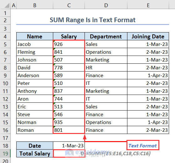
Solution: Changing Text Format to Number Format Directly or Using the VALUE Function

You can change the text format into number format directly or you can use the VALUE function.

• For the first solution, simply select all the cells you want to change the format.
• Click on the triangular-shaped icon at the top of the selected cells and select the Convert to Number
• Your formula is now working fine. You’ll find the whole process in the following video.

• For the second solution, we created a new column titled “Converted to Number” in column F.
• Put the following formula in cell F5 and use the Fill Handle tool for the rest of the values:

• As the values are now converted to number format, we put the following formula in cell C19:

• We changed the sum range to F5:F16 from C5:C16 because they are in number format.

Read More: Excel SUMIFS with Not Equal to Text Criteria

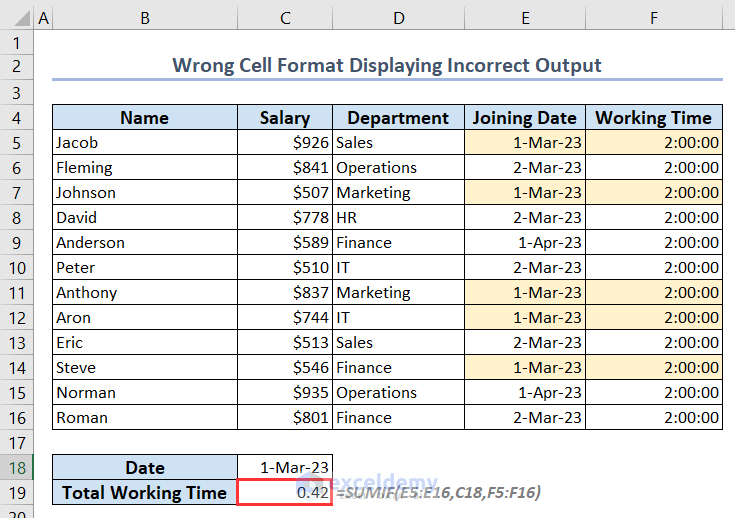
4. Wrong Cell Format Displays Incorrect Output

When you try to add up times values, the SUMIF function might not appear to be working. Here, we want to sum up the working hours of date 1-Mar-23. The working time values are in HH:MM:SS format.

• So I use the formula in cell C19:

• The formula is 100% accurate, however, the result I’m obtaining doesn’t seem right. The answer should be 10:00:00 but it is showing 42. Actually, it is not wrong. Excel converts 1 hour to 1/24 units.  Therefore, 10 hours will equal 0.42.

Solution: Applying the Correct Cell Format

To solve this issue, we have to change the format of cell C19 to the time format.

• Select cell C19 and Right-Click with the mouse.
• Select the Format Cells option to open the Format Cells
• In the Number tab, choose the option Time under Category. Choose 13:30:55 as Type which is our desired format and click on the OK
• You’ll get your desired result. The whole process is shown in the video.

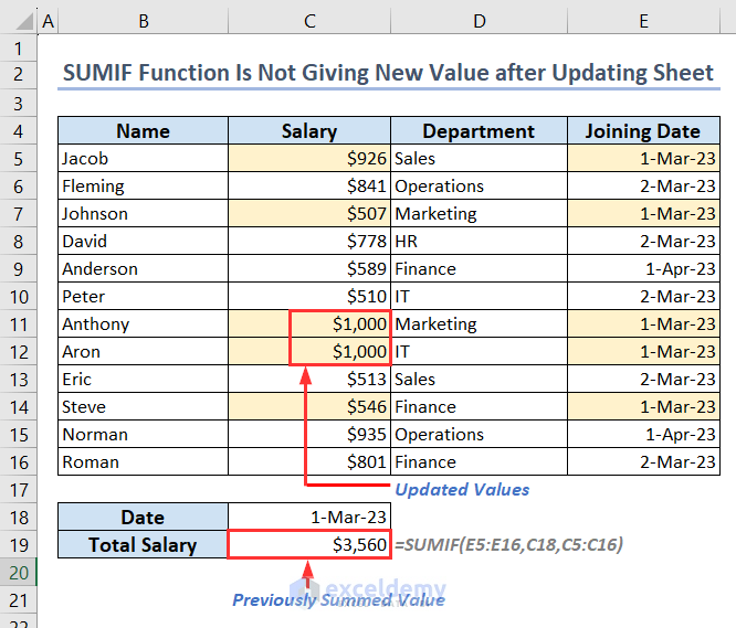
5. SUMIF Function Is Not Giving New Value After Updating Sheet

We have inserted the following formula in cell C19 to get the total salary of employees who joined on the date 1-Mar-23:

Then, we updated 2 salaries of cells C11 and C12 to new values but the summed value in cell C19 remains unchanged.

This may happen when the formula calculation is set to manual.

Solution: Using Keyboard Shortcut or Calculation Options Menu to Recalculate Sheet

We can use the keyboard shortcut or the Calculation Options menu to solve this.

• Just press F9 from the keyboard to recalculate the sheet and the SUMIF function will give the updated result.

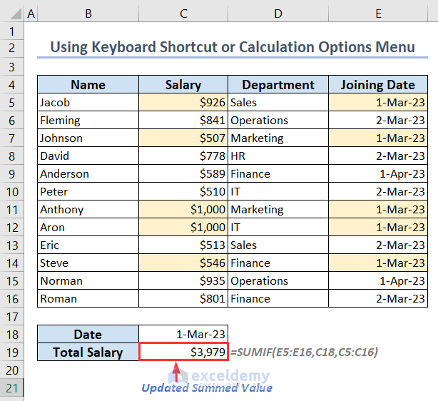
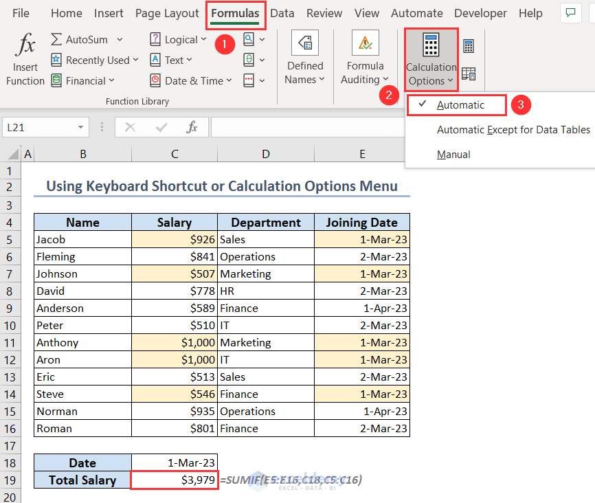
• Or go to the Formulas Select Automatic from the Calculation Options menu.
• Now, whenever you update any values, the SUMIF function will give a new result.

6. SUMIF Function Is Not Working for Multiple Criteria

Only one condition can be used in the SUMIF function’s syntax. You can’t use this function for multiple criteria. We have 2 criteria now based on which we want to sum up the values from the Salary column. Criteria 1 is the department name Sales and Criteria 2 is the joining date. But applying the SUMIF function isn’t giving any results:

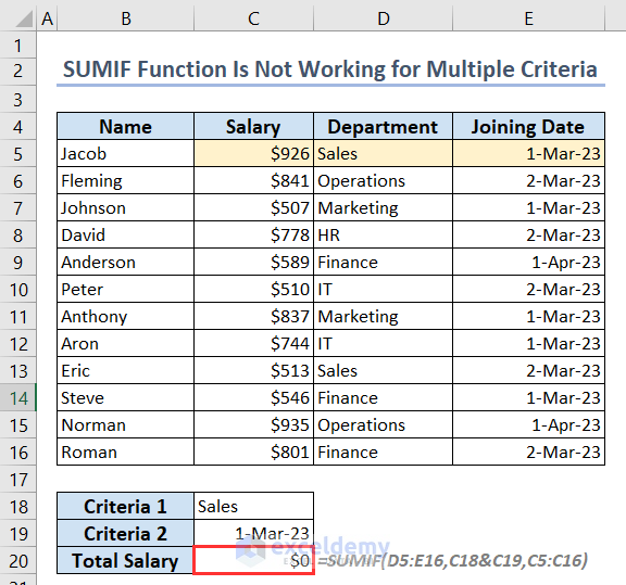
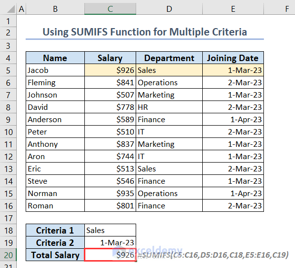
Solution: Using SUMIFS Function for Multiple Criteria

We can use the SUMIFS function for multiple criteria.

• Put the formula in cell C20 instead of the previous formula:

• Here, we first put the sum range as C5:C16. Then, put D5:D16 as the first criteria range and C18 as the first criteria. Similarly put E5:E16 as the second range and C19 as the second criteria.

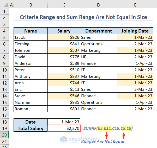
7. Criteria Range and Sum Range Are Not Equal in Size

The range and sum range arguments need to be the same size for the SUMIF formula to function properly; otherwise, you’ll get inaccurate results. We are putting the following formula and getting a false result:

• Here, we put the range as E5:E11 and the sum range as C5:C8 which are not of equal size. That’s why it is giving wrong summed-up values.

Solution: Making Both Ranges of the Same Size

• Write this formula instead in cell C19 by putting the range and sum range arguments of equal size to get the right result:

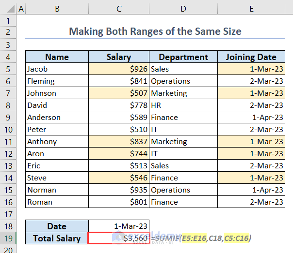
8. SUMIF Function Is Not Working Because Another Workbook Is Close

We have the same dataset in Sheet1 of another workbook titled “Another Workbook”.

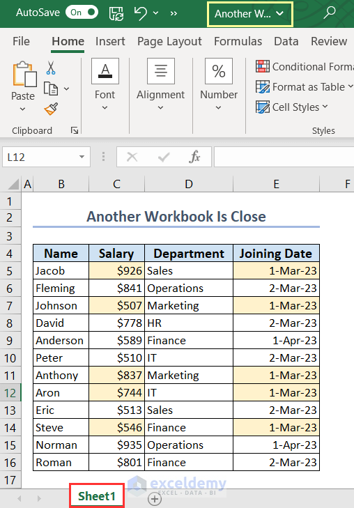
And we want to get the total salary of the date 1-Mar-23 based on this dataset in our existing workbook. So, we entered the following formula and got a #VALUE! error because our “Another Workbook” is closed.

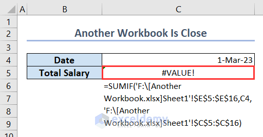
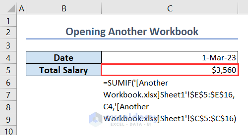
Solution: Opening Another Workbook

• Simply open “Another Workbook” and the formula will work fine.

9. Criteria String Is Greater Than 255 Characters

The last reason Excel SUMIF is not working is when trying to match criteria strings that are longer than 255 characters, the SUMIF function produces inaccurate results. It will give a #VALUE! error. In cell C18, we have a string that is greater than 255 characters. So, putting the following formula in cell C19 is giving the error:

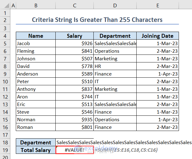
Solution: Take Criteria String Less Than 255 Characters

If you can, make the string shorter. Or you can use the alternative solution which we discussed below instead of the SUMIF function.

The SUMPRODUCT Function in Excel: an Alternative to SUMIF

Use this alternate solution if the SUMIF function is not functioning for any reason at all. In this case, the SUMPRODUCT function is used. We want to get the total salary of the employees who joined on 1-Mar-23. So we put 3 formulas separately using the SUMPRODUCT function. All 3 formulas are correct.

• The first formula is:

• Here, the formula’s –(E5:E16=C18) part generates an array of 1s and 0s, one for each row where E5:E16 and C18 have the same value and one for each row where they don’t. After multiplying each value in the range C5:C16 by its corresponding value in the array, the SUMPRODUCT function returns the sum of those products.
• The second and third formula is the same as the first one. Here, we just change the orientation inside the formula.

Download Practice Workbook

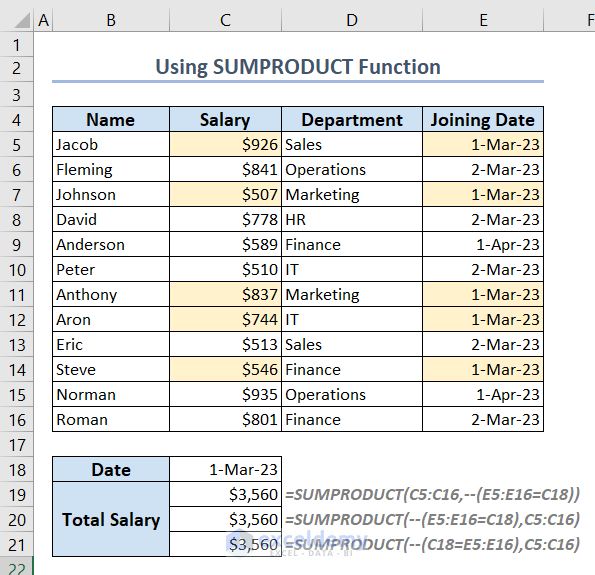
You can download the practice workbook from here and practice on your own.

Conclusion

In this article, we have discussed 9 suitable reasons with solutions when the SUMIF function is not working in Excel. We covered a number of potential concerns, as well as their fixes, from poorly stated criteria arguments to problems with cell formatting. At last, we offer a backup plan via the SUMPRODUCT function if the SUMIF function does not work anyway.

Related Articles

• Excel SUMIF Function for Not Equal Criteria
• How to Use Excel SUMIF with Blank Cells
• How to Use SUMIF Function to Sum Not Blank Cells in Excel

<< Go Back to Excel SUMIF Function | Excel Functions | Learn Excel