Dataset Overview
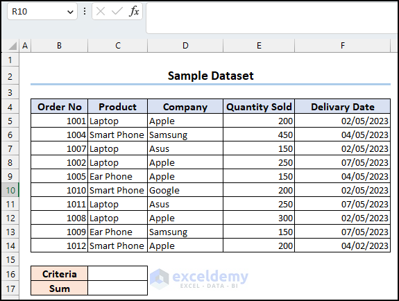
In this tutorial, we’ll explore how to use the SUMIFS function to exclude specific values based on criteria. Let’s consider a dataset containing sales quantities for various tech products, along with their delivery dates. Our goal is to sum the sales quantities of products that do not contain the word Phone in their names, effectively focusing on laptops only.
Example 1 – SUMIFS Function for Not Equal to Partially Matched Text
Suppose we want to sum the sales quantities of laptops (excluding any products with “Phone” in their names).
- Insert the following formula in cell C18:
=SUMIFS(E5:E14,C5:C14,"<>*Phone*")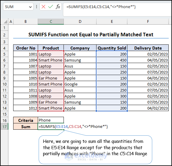
- Press Enter and the formula will add the sales quantity of the laptops only.
How the Formula Works
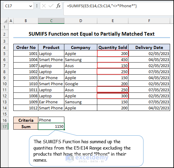
- SUMIFS sums the values in the range E5:E14.
- Before summing, it checks each corresponding value in the range C5:C14.
- The condition is that the product name should not be equal to Phone (using the syntax “<>Phone”).
- The asterisks (*) indicate a partial match, allowing us to exclude products like Ear Phone and Smart Phone.
- The total sum, considering only laptop sales, is 1150.
Handling Multiple Criteria
If you need to address multiple criteria simultaneously, you can extend the formula. For example, to exclude both Phone products and sales from a specific date (e.g., 02/05/2023), use the following formula:
=SUMIFS(E5:E14,C5:C14,"<>*Phone*",F5:F14,"<>02/05/2023")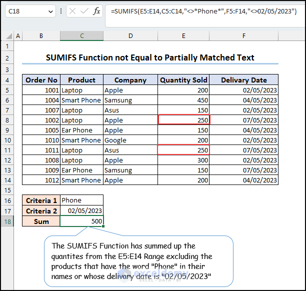
How the Formula Works
The SUMIFS function allows us to add up values from a specified range based on multiple criteria. Let’s break down the components of this function:
- E5:E14: This represents the range of values that we want to sum.
- C5:C14: The second argument specifies the range of values against which we’ll apply the first criterion.
- “<>Phone”: The third argument defines the first criterion. It instructs the function to include values from the range that do not contain the text “Phone.” The “<>” operator means “not equal to,” and the asterisks (*) act as wildcards, allowing any text before and after the word “Phone.”
- F5:F14: The fourth argument is the range of values against which we’ll apply the second criterion.
- “<>02/05/2023”: The fifth argument sets the second criterion. It includes values from the range that are not equal to the date “02/05/2023.”
Read More: Excel SUMIF Function for Not Equal Criteria
Example 2 – Using SUMIFS to Exclude Exactly Matched Text
In this example, we want to add up the values from the Quantity Sold column that do not match either Smart Phone in the Product column or the date 04/05/2023 in the Delivery Date column.
- Insert the following formula into cell C18 to achieve this result:
=SUMIFS(E5:E14,C5:C14,"<>Smart Phone",F5:F14,"<>04/05/2023")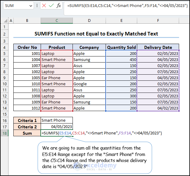
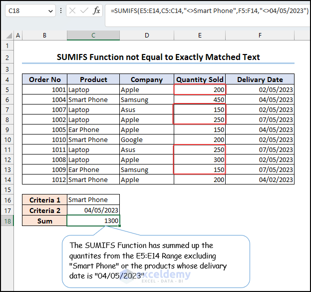
- When we press Enter, the formula will sum the sales quantity of products excluding Smart Phone and those with a delivery date other than 04/05/2023.
How the Formula Works
-
- The formula adds up the sales quantities from the E5:E14 range.
- It checks the corresponding values in the C5:C14 range against the condition that the product name should not be equal to Smart Phone.
- Simultaneously, it evaluates the F5:F14 range, excluding any dates equal to 04/05/2023”
By combining these criteria, we obtain the desired result.
Example 3 – Using SUMIFS with Cell References for Text Exclusions
In this scenario, we’ll utilize cell references for criteria texts instead of hard-coding them directly into the formula. This approach provides flexibility, as we can easily adjust the criteria by changing the cell references.
- Enter the following formula into cell C18 to achieve our goal:
=SUMIFS(E5:E14,D5:D14,"<>"&C16,C5:C14,"<>"&C17)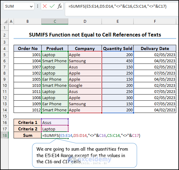
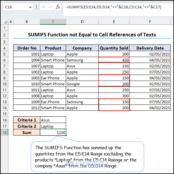
- As soon as we press Enter, the formula will sum the sales quantities of products that are either not labeled as Laptop or do not belong to the brand Asus.
How the Formula Works
- The formula adds up the sales quantities from the E5:E14 range.
- It checks the corresponding values in the D5:D14 range against the condition that the company name should not be equal to Asus.
- Simultaneously, it evaluates the C5:C14 range, excluding any products labeled as Laptop.
By using cell references, we maintain flexibility and adaptability in our calculations.
Example 4 – Using SUMIFS with Non-Empty Delivery Dates
In this example, we want to calculate the total sales quantity for products with recorded delivery dates. Specifically, we’ll use the SUMIFS function to achieve this.
1. Objective: Calculate the total sales quantity for products with non-blank delivery dates.
2. Formula:
- Insert the following formula into cell C16:
=SUMIFS(E5:E14,F5:F14,"<>")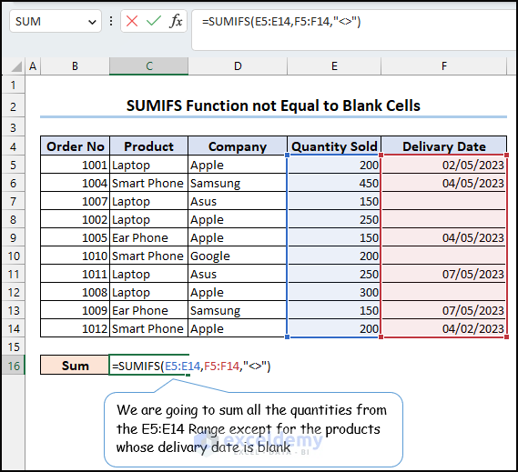
- As soon as we press Enter, the formula will add the sales quantity of the products whose delivery dates are not blank.

How the Formula Works
- Explanation:
- E5:E14: This range contains the sales quantities for various products.
- F5:F14: This range corresponds to the delivery dates.
- “<>”: This criterion ensures that we include only non-empty cells (i.e., delivery dates that are not blank).
3. Result:
- Press Enter after entering the formula, it will sum up the sales quantities for products with non-empty delivery dates.
In summary, the SUMIFS function adds up the sales quantities (from range E5:E14) for products whose delivery dates (in range F5:F14) are not empty.
Read More: How to Use Excel SUMIF with Blank Cells
Download Practice Workbook
You can download the practice book here.
Related Articles
- How to Use SUMIF Function to Sum Not Blank Cells in Excel
- Excel SUMIF Not Working
- [Fixed!] Excel SUMIF with Wildcard Not Working
<< Go Back to Excel SUMIF Function | Excel Functions | Learn Excel
Get FREE Advanced Excel Exercises with Solutions!

Sumifs based on partial Numeric codes i.e. 1020 in 1020-3052 1020-4050.
Hello, Khurram Javed!
As of the latest version of Excel, the SUMIFS function doesn’t support partial matches with numbers directly. If your codes contain alphanumeric characters then the formula works perfectly. Because Excel doesn’t recognize them as “number” format.
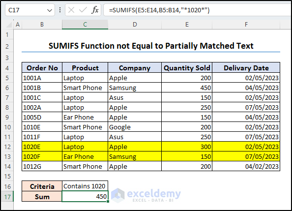
If the range B5:B14 contains numeric values only (i.e. 102054), the function will return a #VALUE! error saying wrong data type.
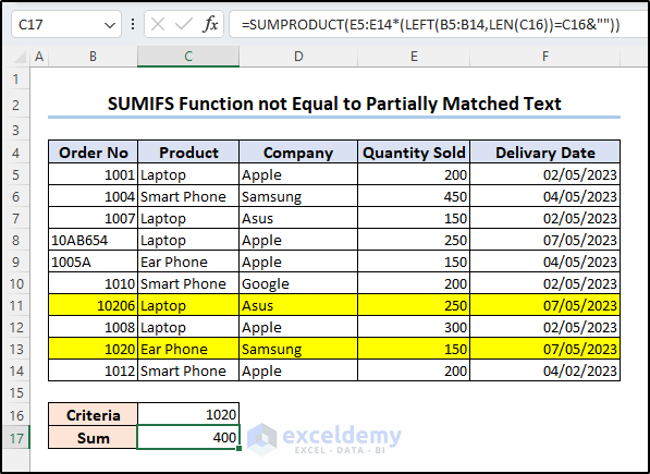
However, if you are only concerned with the result and not with the formula, there is a workaround for that.